Environmental Data Analysis and Visualization
Wrangling in the Tidyverse
A brief reminder
This course deals with the representation of data as a means to communicating about important issues. Our ability to consider a wide and topical range of data representations depends on respect for each other and a commitment to our shared motivation to learn.
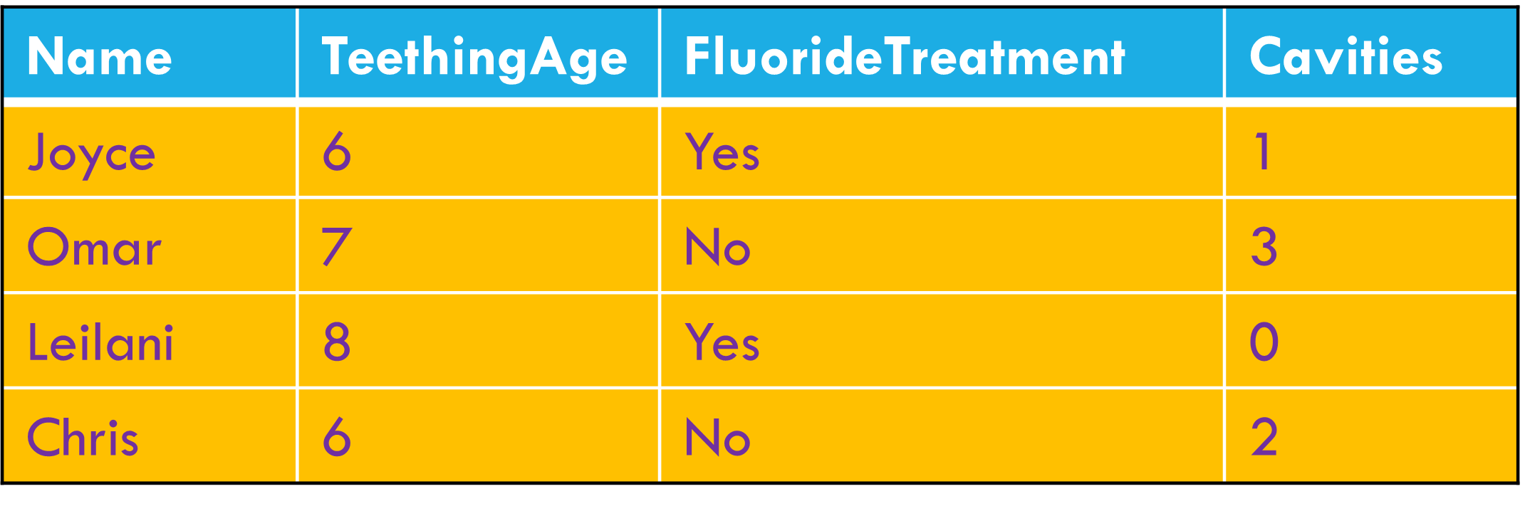
Data
Data are individual pieces of information.
Datasets
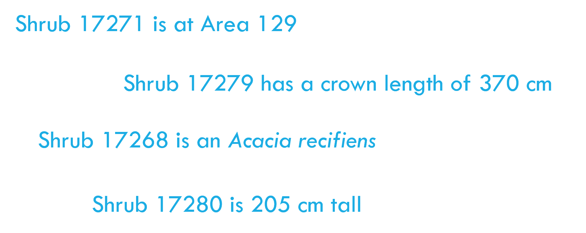
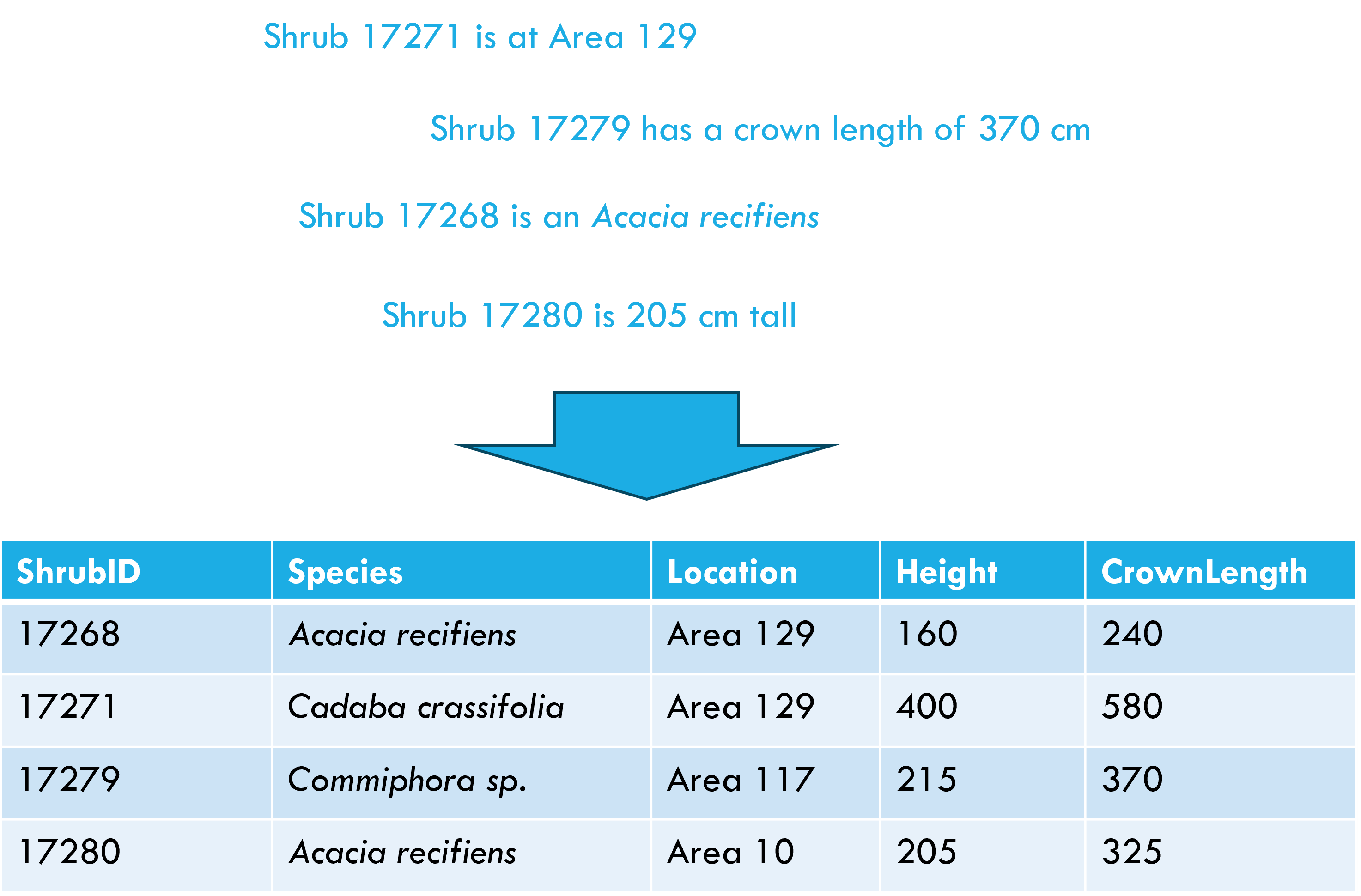
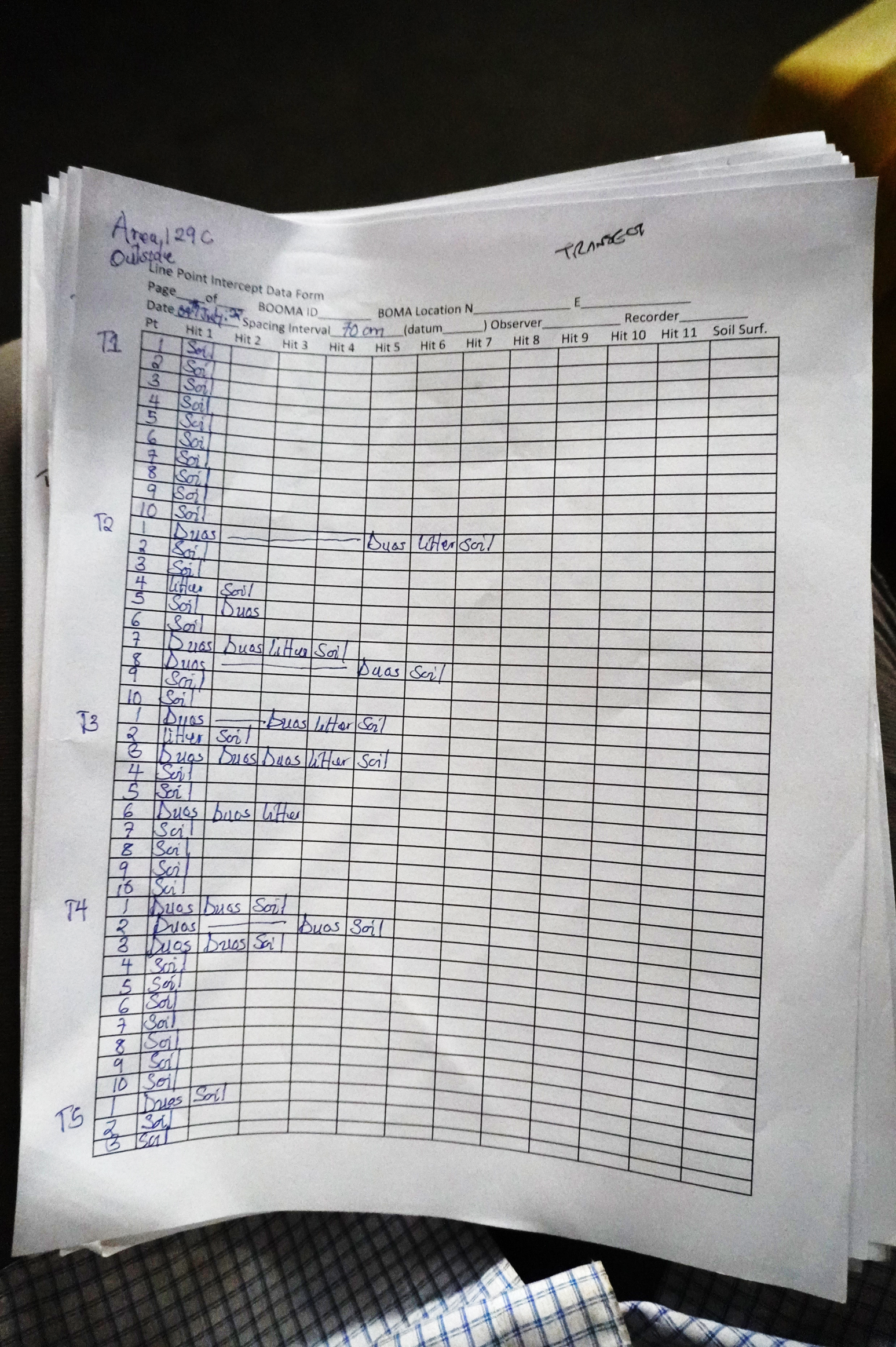
Data in the field
Data in the field
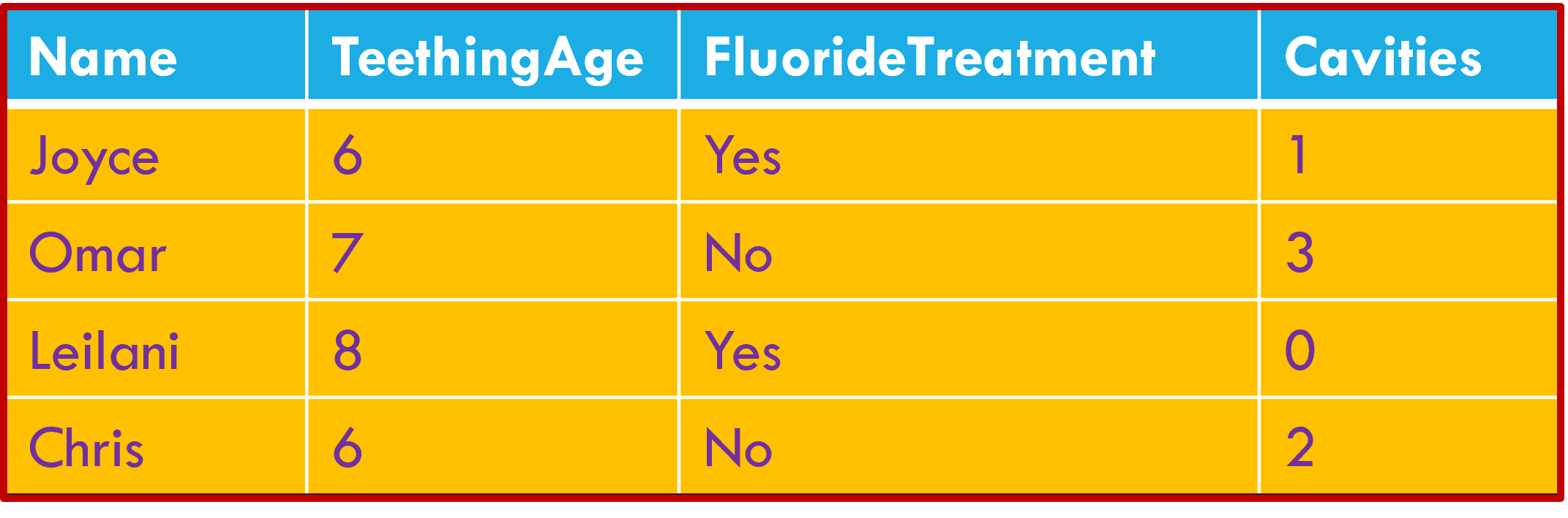
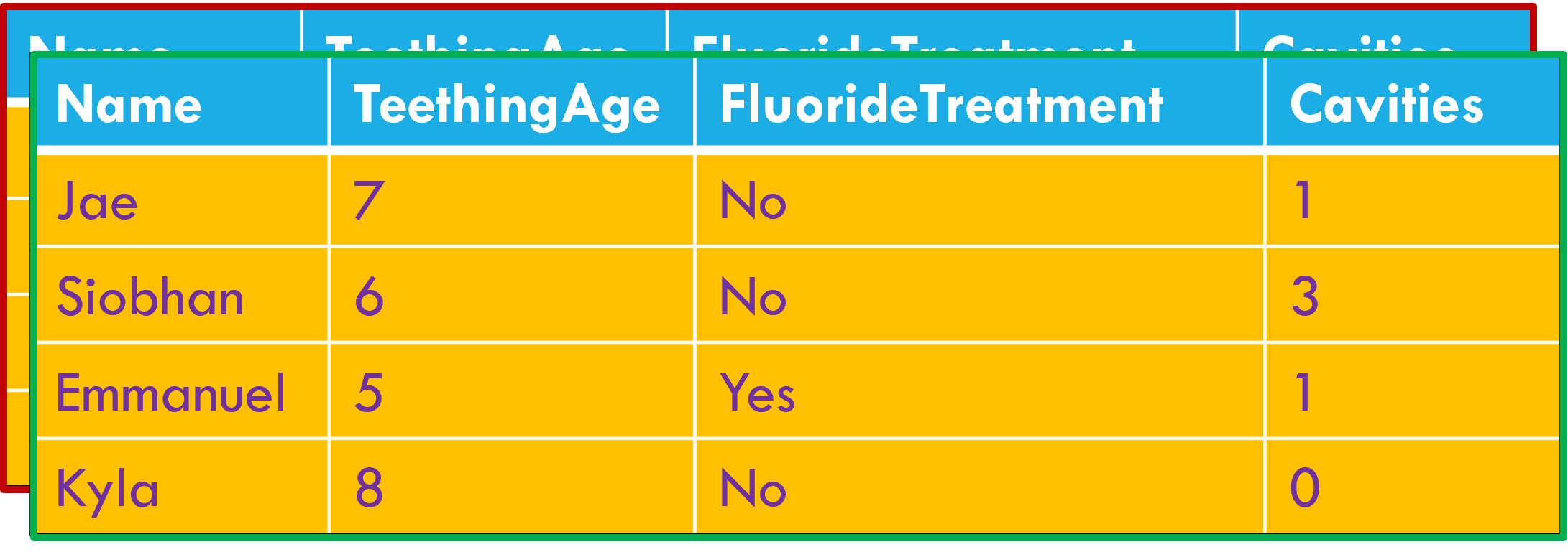
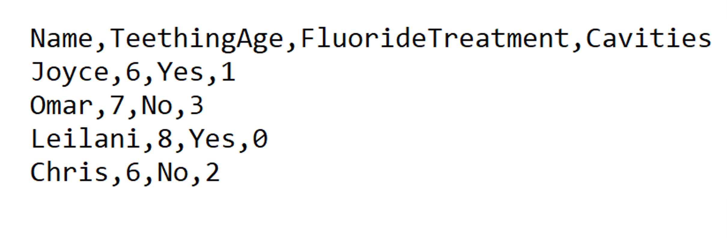
Messy data
The process of data entry is often designed and conducted with limited consideration given to the process of data analysis.
https://openscapes.org/blog/2020-10-12-tidy-data/
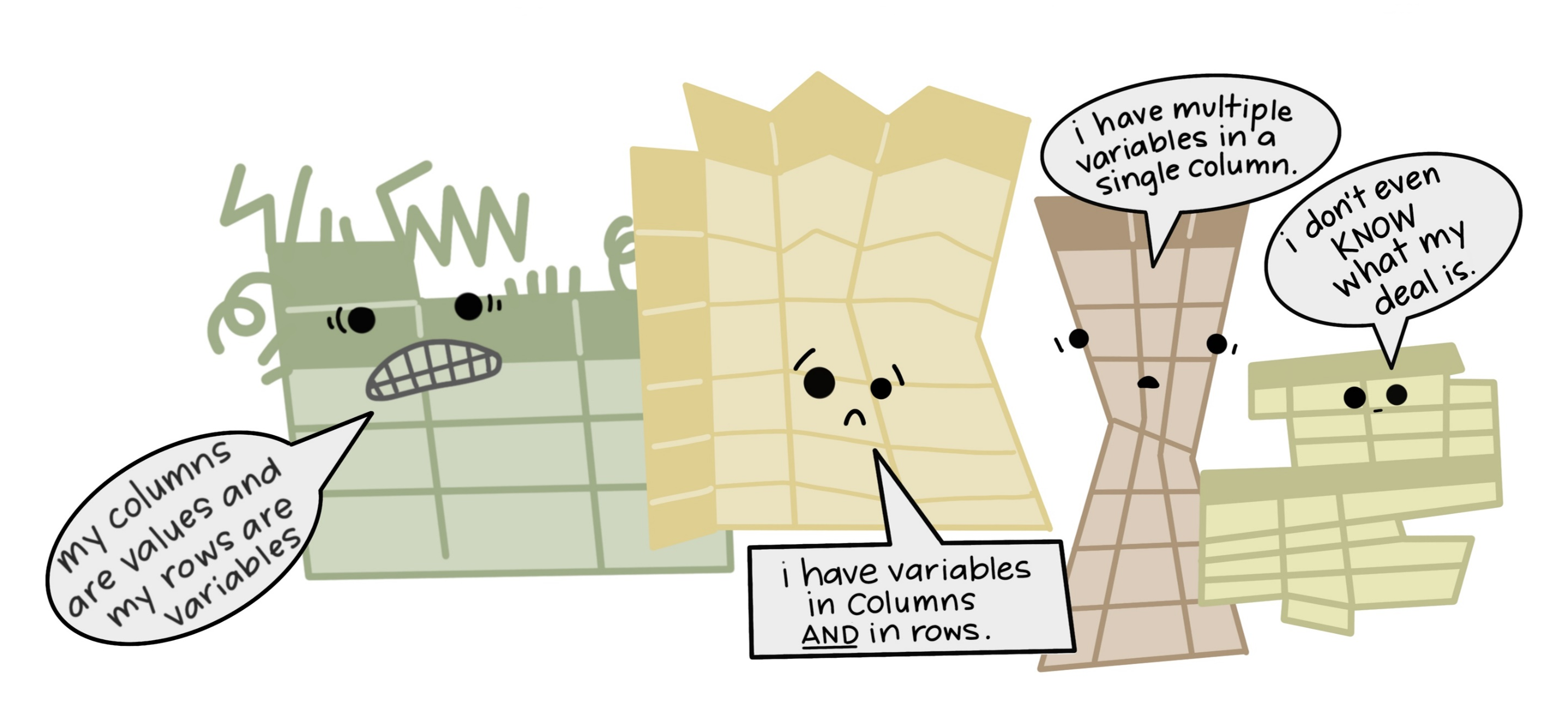
Tidy data principles
Each variable forms a column
Each observation forms a row
Each cell contains a single value
After Wickham, H. 2014. Tidy data. The Journal of Statistical Software 59.
Ease of identification and re-use
Data wrangling: the big three
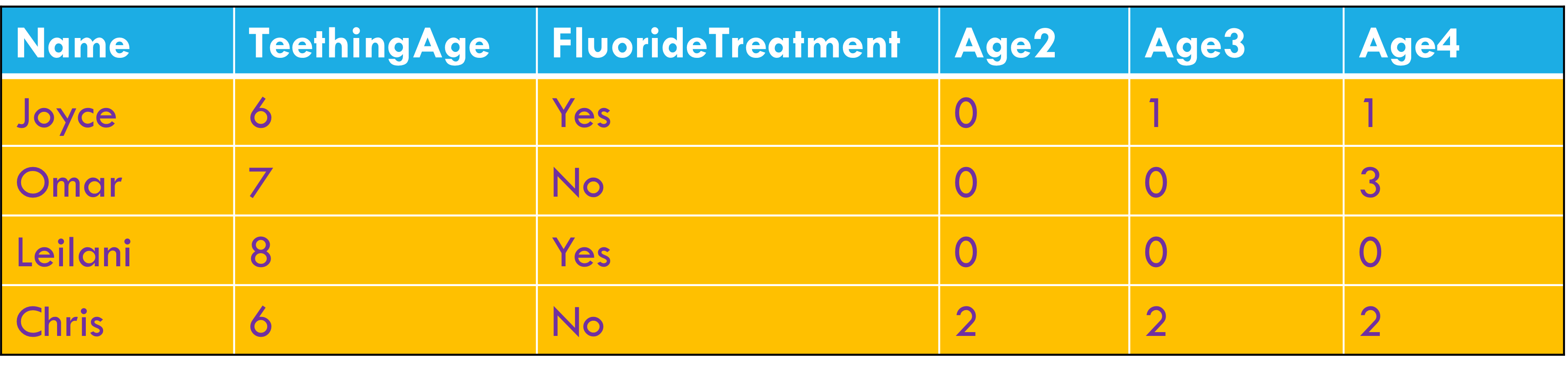
Column headers are values, not variable names.
Data wrangling: the big three
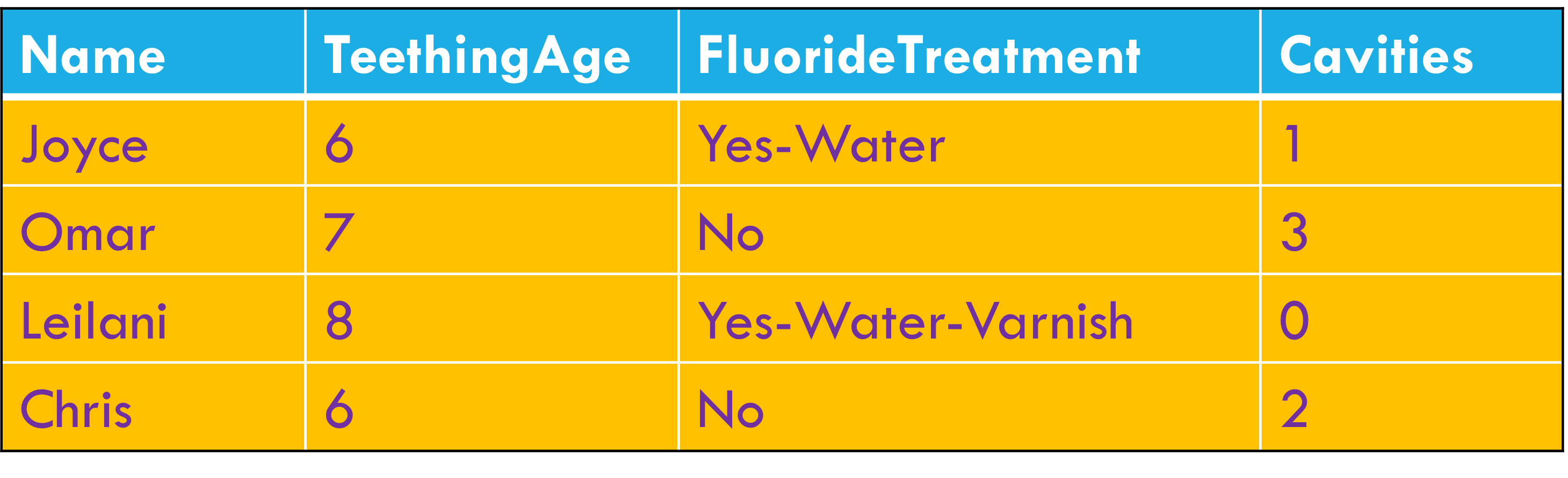
Multiple variables are stored in a single column.
Data wrangling: the big three
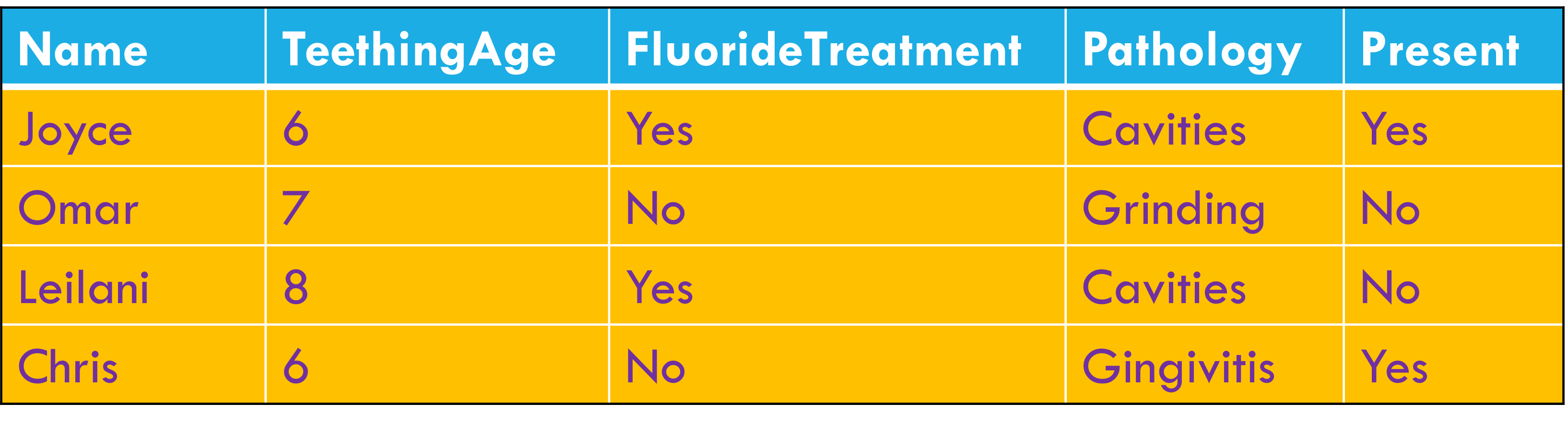
Variables stored in both rows and columns.
Pipes in R
The pipe operator %>% allows us to combine multiple functions into an ordered set of transformations
Pipes in R
# A tibble: 32,735 × 16
    year month   day dep_time dep_delay arr_time arr_delay carrier tailnum
   <int> <int> <int>    <int>     <dbl>    <int>     <dbl> <chr>   <chr>
 1  2013     6    30      940        15     1216        -4 VX      N626VA
 2  2013     5     7     1657        -3     2104        10 DL      N3760C
 3  2013    12     8      859        -1     1238        11 DL      N712TW
 4  2013     5    14     1841        -4     2122       -34 DL      N914DL
 5  2013     7    21     1102        -3     1230        -8 9E      N823AY
 6  2013     1     1     1817        -3     2008         3 AA      N3AXAA
 7  2013    12     9     1259        14     1617        22 WN      N218WN
 8  2013     8    13     1920        85     2032        71 B6      N284JB
 9  2013     9    26      725       -10     1027        -8 AA      N3FSAA
10  2013     4    30     1323        62     1549        60 EV      N12163
# ℹ 32,725 more rows
# ℹ 7 more variables: flight <int>, origin <chr>, dest <chr>, air_time <dbl>,
#   distance <dbl>, hour <dbl>, minute <dbl>
Pipes in R
%>% filter (month== 1 )
# A tibble: 2,610 × 16
    year month   day dep_time dep_delay arr_time arr_delay carrier tailnum
   <int> <int> <int>    <int>     <dbl>    <int>     <dbl> <chr>   <chr>
 1  2013     1     1     1817        -3     2008         3 AA      N3AXAA
 2  2013     1    23     2024        37     2141        29 EV      N17115
 3  2013     1    15     1626        -3     1941        10 B6      N594JB
 4  2013     1    17      626        -4      846         3 US      N554UW
 5  2013     1     8      902        -3     1006       -17 B6      N281JB
 6  2013     1    15     1947       167     2241       171 AA      N5EGAA
 7  2013     1     1     1454        -4     1554       -21 EV      N11544
 8  2013     1    30     1306        -9     1430        -1 EV      N13969
 9  2013     1     4     1942        -3     2249       -40 B6      N637JB
10  2013     1     8     1859        -6     2158       -27 AA      N322AA
# ℹ 2,600 more rows
# ℹ 7 more variables: flight <int>, origin <chr>, dest <chr>, air_time <dbl>,
#   distance <dbl>, hour <dbl>, minute <dbl>
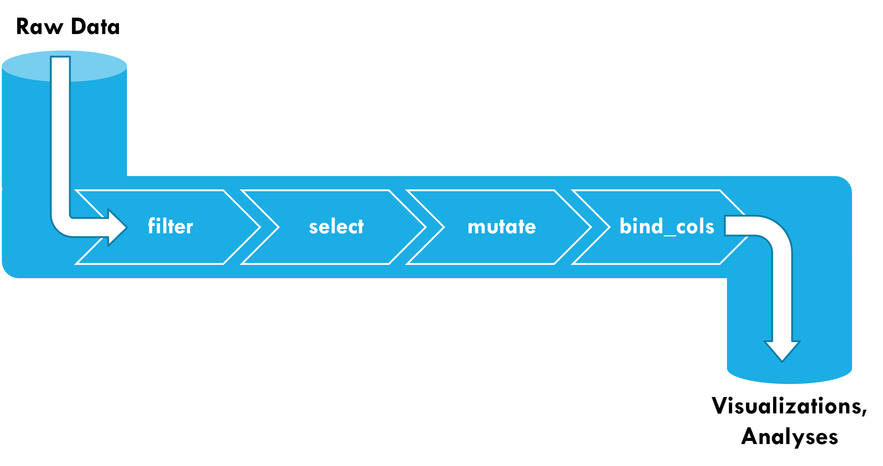
Data pipelines
Pipelines start with raw data (e.g., tibble) as the input
This table is passed as the first argument to the next function (so they don’t need the data argument)
The result of a pipeline is a dataset that can be fed into visualizations and analysis.
Data pipelines
Data pipelines
%>% mutate (speed = distance / air_time * 60 ) %>% select (year: day,dep_time,carrier,flight,speed) %>% filter (month== 1 ) %>% unite (col= "Date" ,c (month,day,year),sep= "/" )
# A tibble: 2,610 × 5
   Date      dep_time carrier flight speed
   <chr>        <int> <chr>    <int> <dbl>
 1 1/1/2013      1817 AA         353  319.
 2 1/23/2013     2024 EV        4412  319.
 3 1/15/2013     1626 B6         369  414
 4 1/17/2013      626 US        1433  311.
 5 1/8/2013       902 B6          56  340.
 6 1/15/2013     1947 AA         575  396.
 7 1/1/2013      1454 EV        4390  363.
 8 1/30/2013     1306 EV        4120  277.
 9 1/4/2013      1942 B6         645  466.
10 1/8/2013      1859 AA          21  441.
# ℹ 2,600 more rows
Activity: Going with the directional movement of a fluid
Working in pairs or small groups, use the different tidyverse functions to create a pipeline to wrangle raw data into the desired form
Datasets will come from Canvas and the modeldata package
Use cheatsheets on Canvas for function descriptions
Example 1
Body mass and flipper length for penguins from Biscoe and Dream islands with a body mass over 400 grams.
Example 2
Price, number of baths, and square meters for three-bedroom homes in the Roseville, Orangevale, and Citrus Heights neighborhoods of Sacramento .
Example 3
ID Number, Diameter in mm, and number of rings on top 100 abalone by ring count.
Example 3
<- read_csv ("data/abalone.csv" )%>% mutate (diameter_mm= diameter * 200 ) %>% select (...1 ,diameter_mm,rings) %>% slice_max (order_by= rings,n= 100 )
# A tibble: 136 × 3
    ...1 diameter_mm rings
   <dbl>       <dbl> <dbl>
 1   481         117    29
 2  2109         107    27
 3  2210          93    27
 4   295          99    26
 5  2202          98    25
 6  3150         108    24
 7  3281         108    24
 8   314          94    23
 9   315          97    23
10   502         104    23
# ℹ 126 more rows
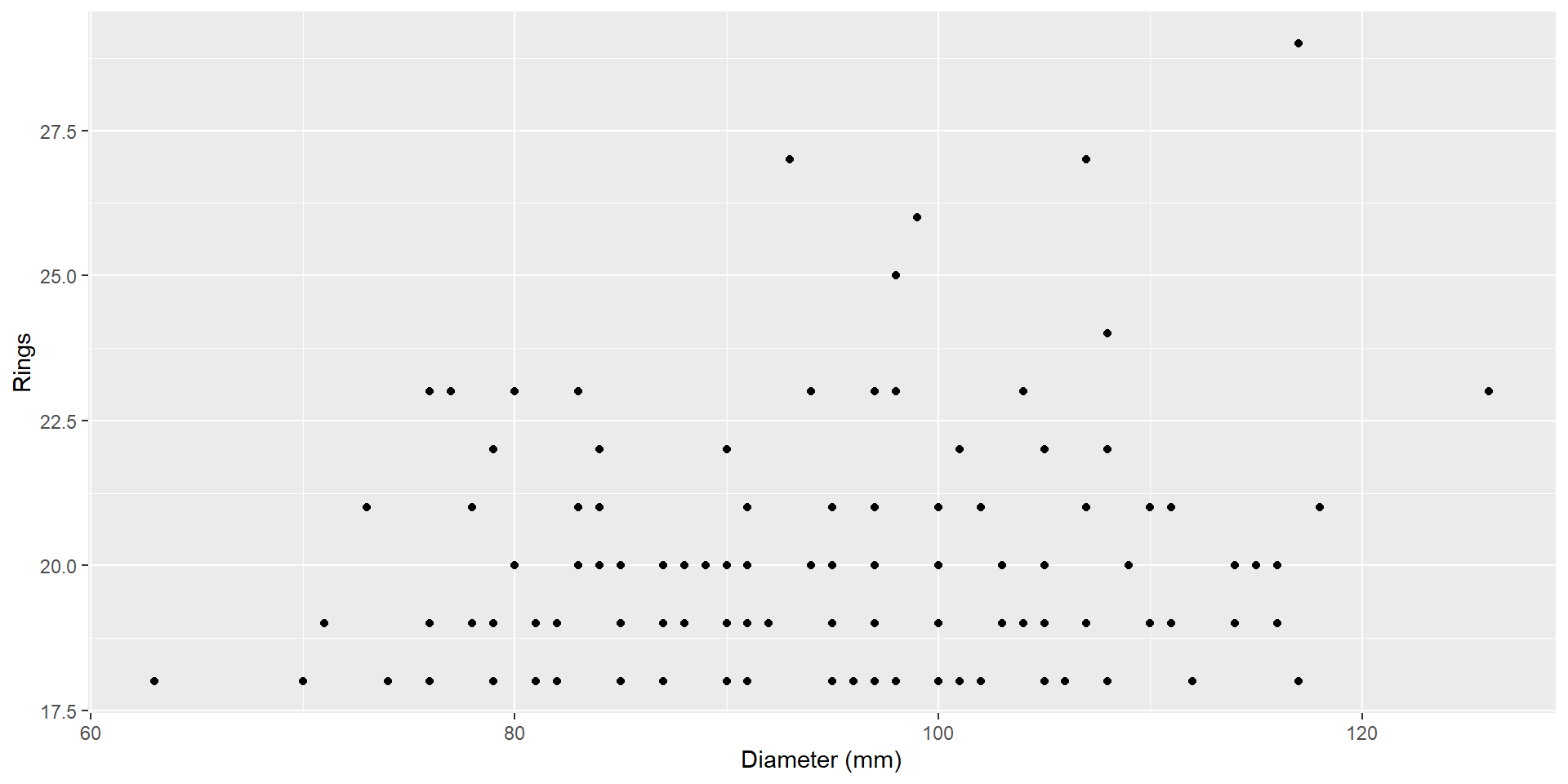
Can I use pipes with ggplot2?
Can I use pipes with ggplot2?
YES!
%>% mutate (diameter_mm= diameter * 200 ) %>% select (...1 ,diameter_mm,rings) %>% slice_max (order_by= rings,n= 100 ) %>% ggplot (aes (x= diameter_mm,y= rings)) + geom_point () + labs (x= "Diameter (mm)" ,y= "Rings" )
Can I use pipes with Base R?
Can I use pipes with Base R?
YES!
%>% mutate (wholeWeight= weight.whole * 200 ) %>% mutate (shuckedWeight= weight.shucked * 200 ) %>% select (wholeWeight,shuckedWeight) %>% colSums ()
  wholeWeight shuckedWeight
     692331.2      300215.6
Can I use pipes with Base R?
YES!*
%>% mutate (wholeWeight= weight.whole * 200 ) %>% mutate (shuckedWeight= weight.shucked * 200 ) %>% select (wholeWeight,shuckedWeight) %>% sum (wholeWeight)
Error: object 'wholeWeight' not found
Can I use pipes with Base R?
YES!*
%>% mutate (wholeWeight= weight.whole * 200 ) %>% mutate (shuckedWeight= weight.shucked * 200 ) %>% select (wholeWeight,shuckedWeight) %>% sum (.$ wholeWeight)}
*certain rules apply when first argument is not the first argument, or when referencing column names
Can I use pipes for modeling data?
YES!
%>% mutate (diameter_mm= diameter * 200 ) %>% select (...1 ,diameter_mm,rings) %>% lm (rings ~ diameter_mm, data= .) %>% summary ()
Call:
lm(formula = rings ~ diameter_mm, data = .)

Residuals:
    Min      1Q  Median      3Q     Max
-5.1868 -1.6932 -0.7200  0.9066 15.9999

Coefficients:
            Estimate Std. Error t value Pr(>|t|)
(Intercept) 2.318574   0.172737   13.42   <2e-16 ***
diameter_mm 0.093350   0.002057   45.37   <2e-16 ***
---
Signif. codes:  0 '***' 0.001 '**' 0.01 '*' 0.05 '.' 0.1 ' ' 1

Residual standard error: 2.639 on 4175 degrees of freedom
Multiple R-squared:  0.3302,    Adjusted R-squared:  0.3301
F-statistic:  2059 on 1 and 4175 DF,  p-value: < 2.2e-16
Coursekeeping
Coding exercise 2 is now available on Canvas, due November 6!
the-decoder.com