Environmental Data Analysis & Visualization
Warm-up activity
Create a file system for this week and add a new Quarto document for today’s lecture.
Download the GSS.csv dataset and load it into R as a tibble
Have a look at sparts and income16 variables: what might these different values represent?
Go to the links on Canvas and take a look at the metadata for each variable. Can you think of a way to modify the data to get a meaningful plot out of it?
Sensor Dataset of the day
General Social Survey

Data
Data are individual pieces of information.
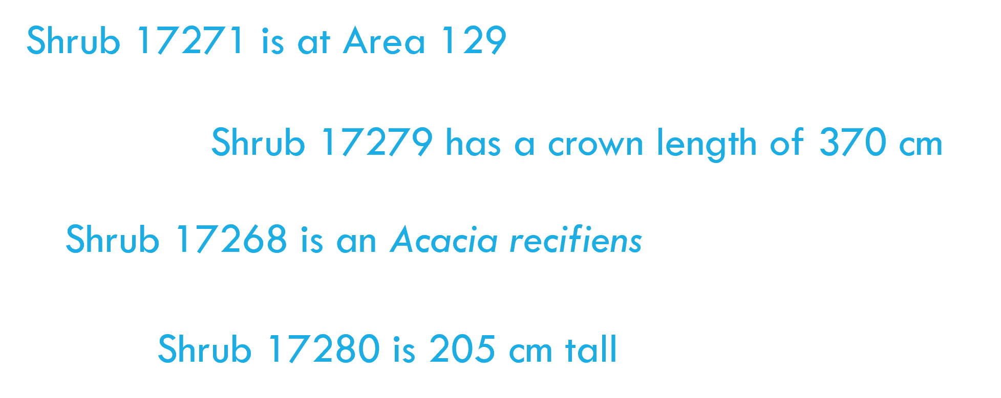
Datasets
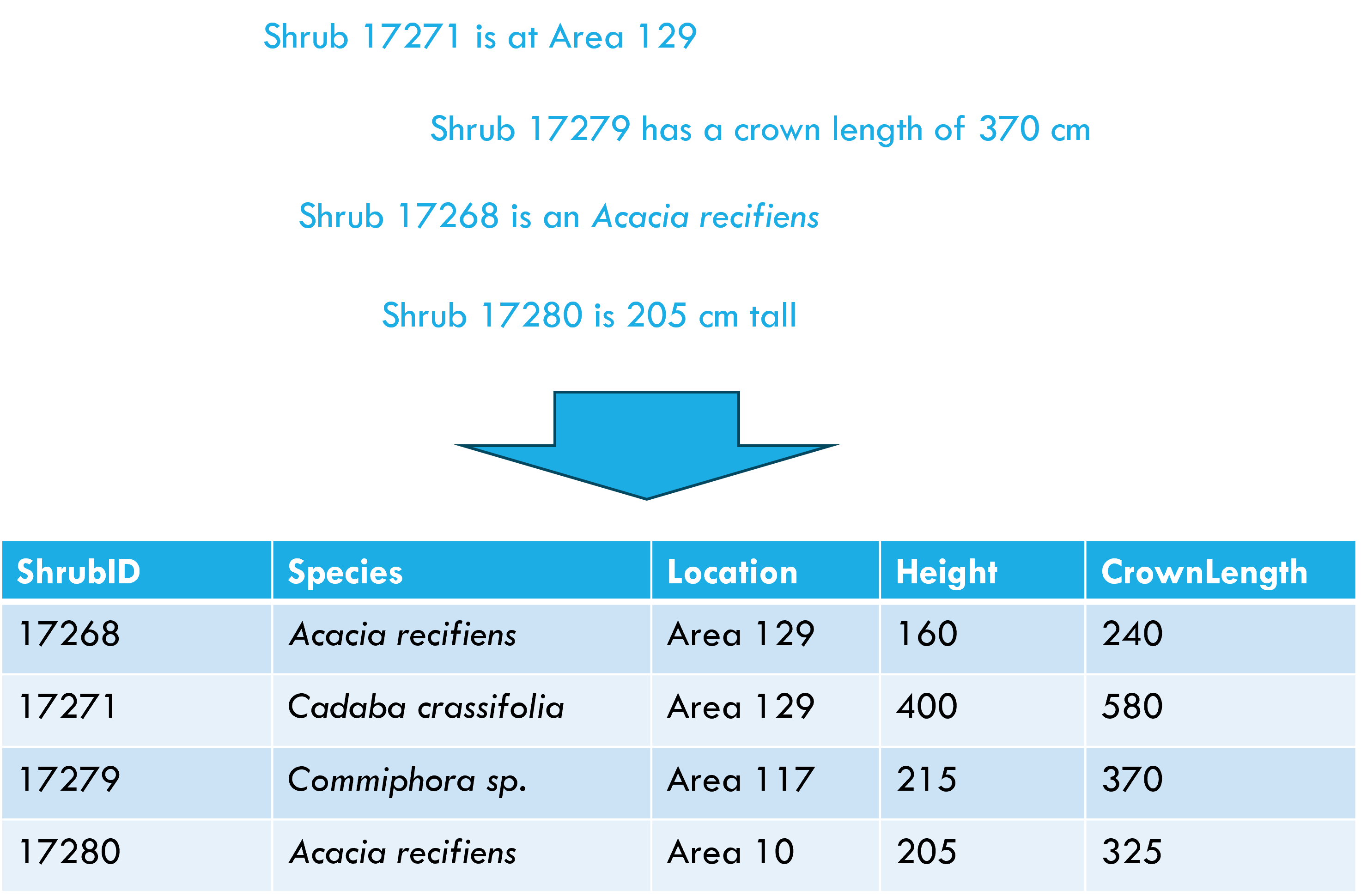
Data in the field

Data in the field
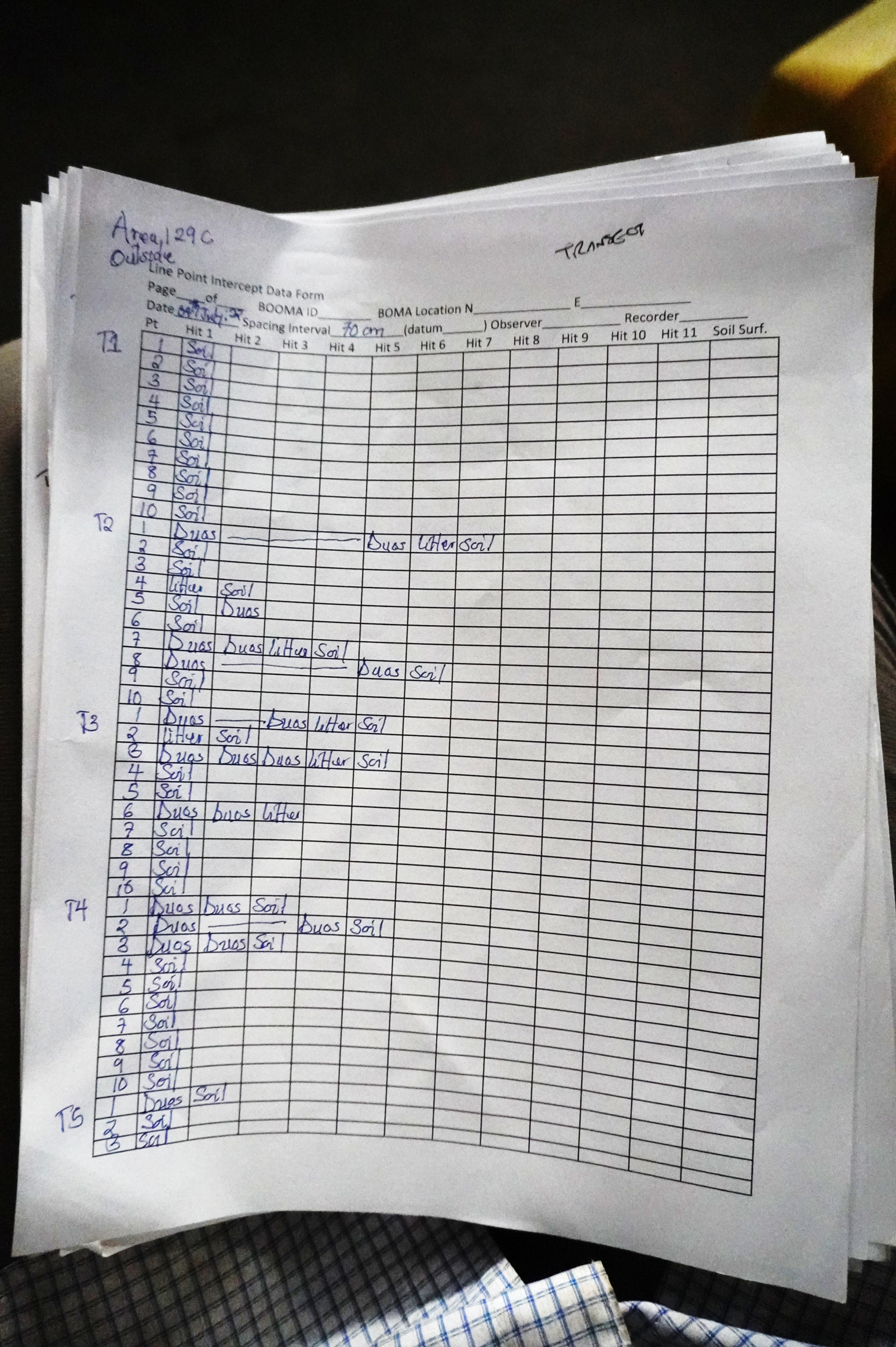
Messy data
The process of data entry is often designed and conducted with limited consideration given to the process of data analysis.
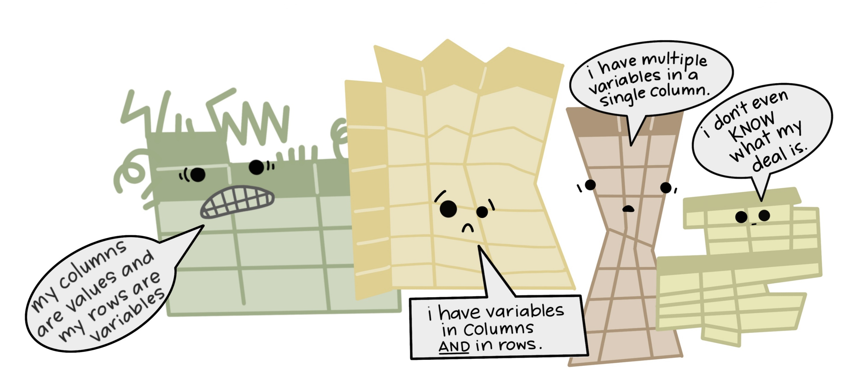
https://openscapes.org/blog/2020-10-12-tidy-data/
Tidy data principles
Each variable forms a column
Each observation forms a row
Each cell contains a single value

After Wickham, H. 2014. Tidy data. The Journal of Statistical Software 59.
Vectorization


Querying


Consistency
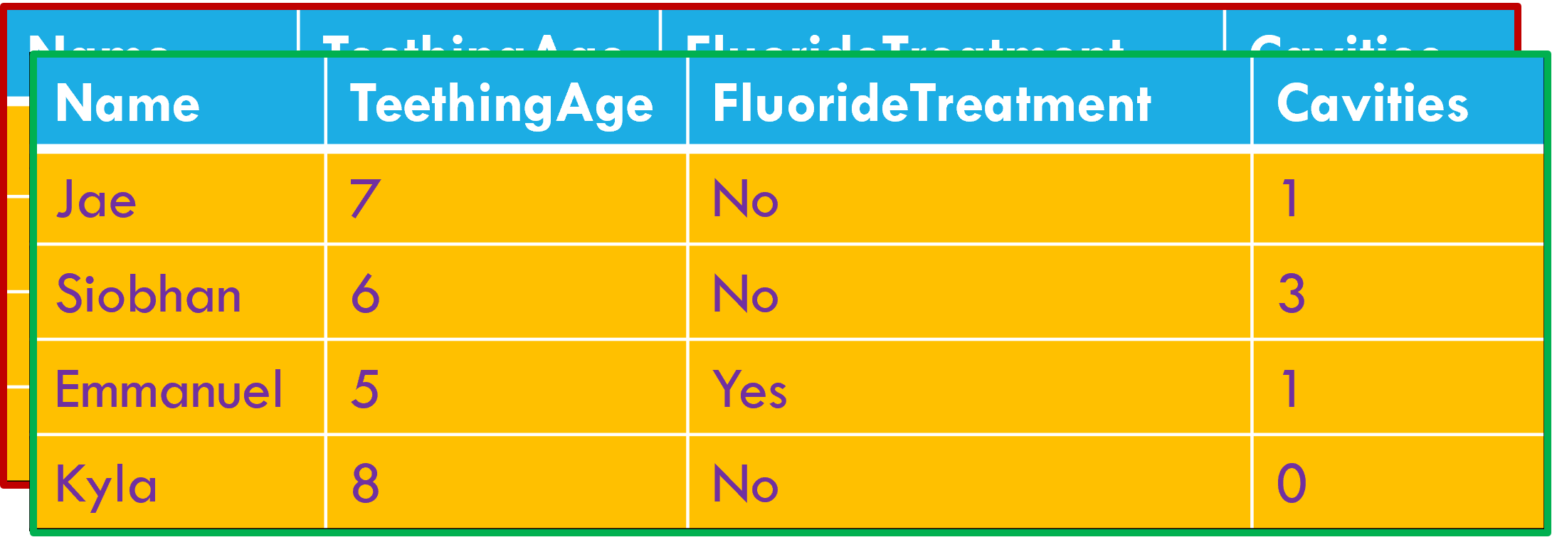

Ease of identification and re-use

Activity: Making a mess of data
With the sticky notes you’ve been given, complete the data table that’s been started on the door to the data lab. Use Google Maps or similar to estimate transportation times.

friendsofthefells.org
Exploring the data
Compare university year to drive time.
Exploring the data
Compare university year to drive time.

Exploring the data
Compare university year to drive time.

Exploring the survey data
Compare university year to public transit time.

Exploring the survey data
Compare university year to public transit time.

Exploring the survey data
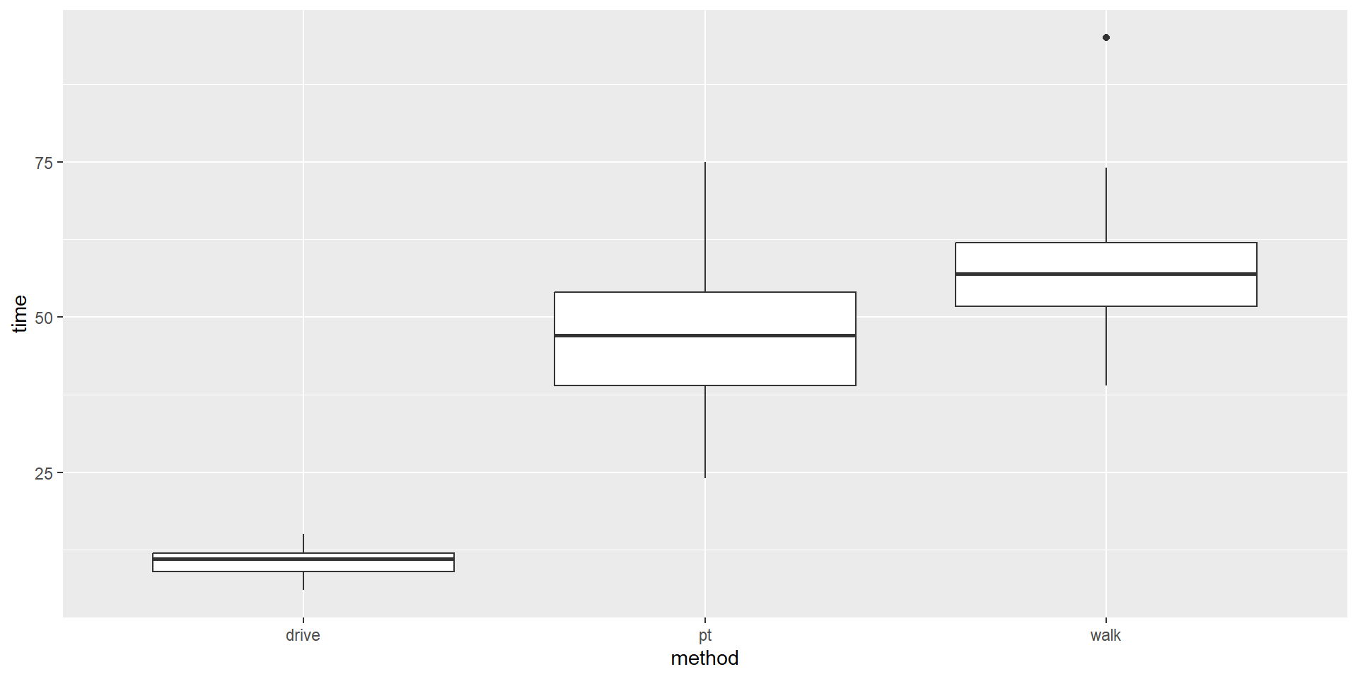
Compare mode of transportation to time spent in transit.

Exploring the survey data
Compare mode of transportation to time spent in transit.

Data wrangling: the big three
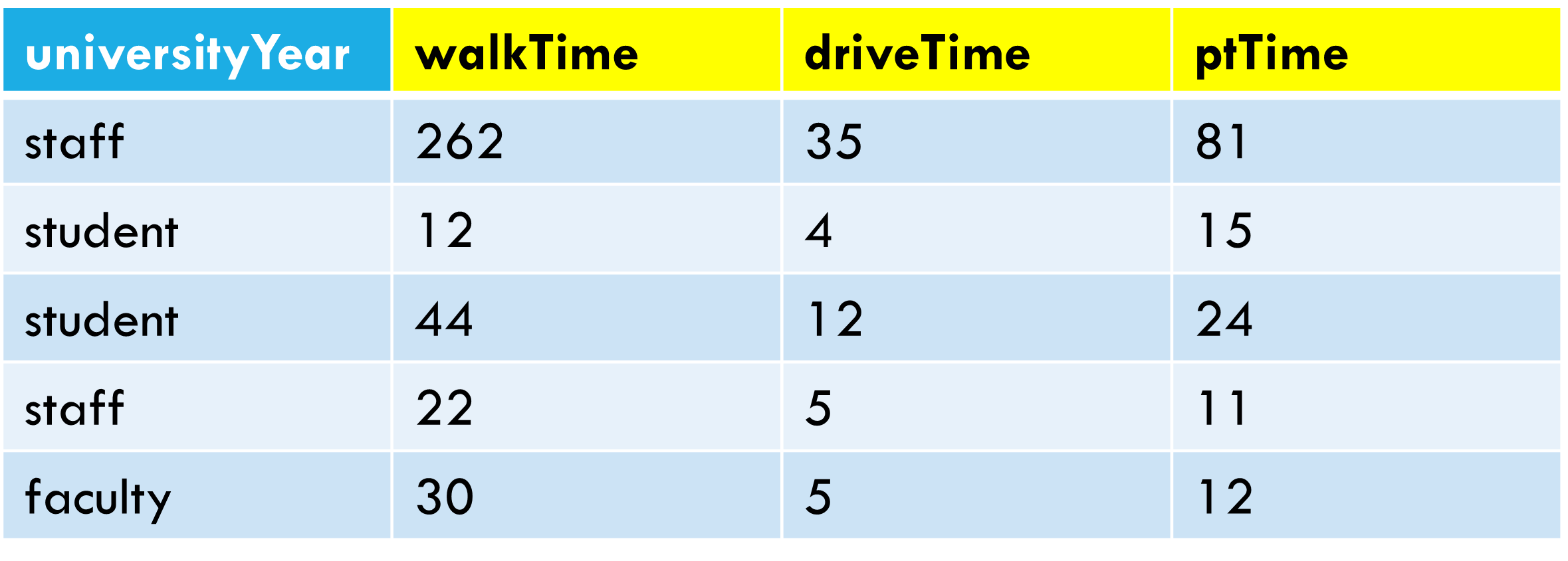
Column headers are values, not variable names.

Data wrangling: the big three
Multiple variables are stored in a single column.

Data wrangling: the big three
Variables stored in both rows and columns.

Into the tidyverse


Data wrangling in the tidyverse
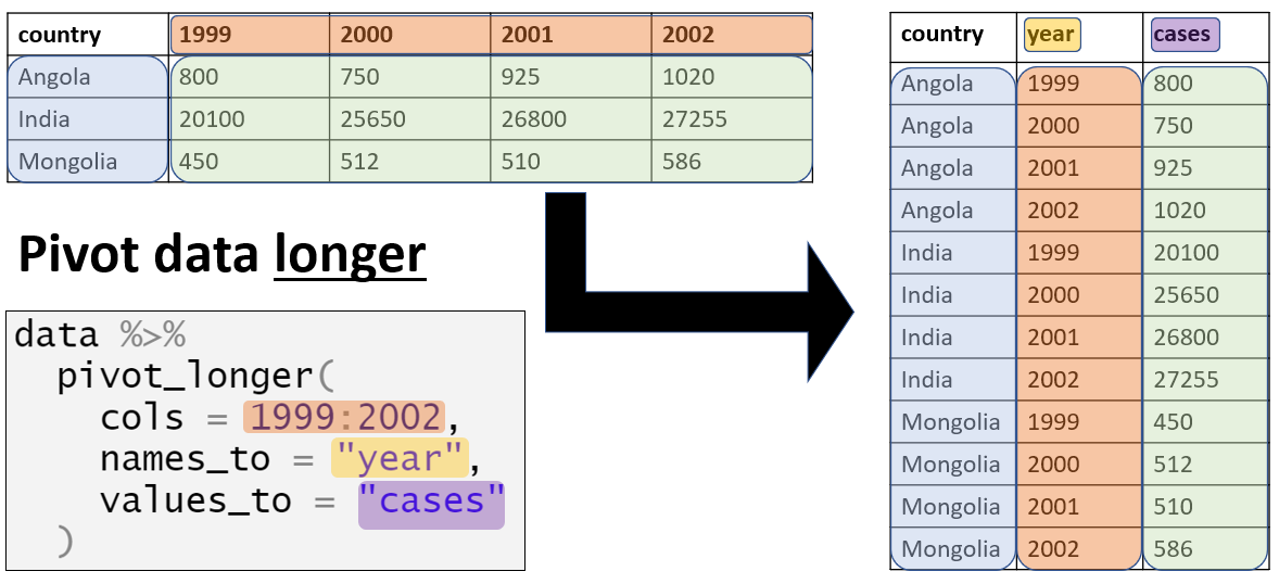
epirhandbook.com/en/pivoting-data.html
Data wrangling in the tidyverse
# A tibble: 64 × 4
   universityYear walkTime driveTime ptTime
   <chr>             <dbl>     <dbl>  <dbl>
 1 first                65        12     37
 2 first                60        12     51
 3 first                66        10     33
 4 first                58        14     60
 5 first                70        12     44
 6 first                62        11     40
 7 first                62        11     52
 8 first                57         9     60
 9 first                66        11     50
10 first                66        11     55
# ℹ 54 more rows
Data wrangling in the tidyverse
fellsData2<-pivot_longer(
  data=fellsData,
  cols=walkTime:ptTime,
  names_to="method",
  values_to="time"
  )
fellsData2
# A tibble: 192 × 3
universityYear method time
<chr> <chr> <dbl>
1 first walkTime 65
2 first driveTime 12
3 first ptTime 37
4 first walkTime 60
5 first driveTime 12
6 first ptTime 51
7 first walkTime 66
8 first driveTime 10
9 first ptTime 33
10 first walkTime 58
# ℹ 182 more rowsData wrangling in the tidyverse
fellsData2<-pivot_longer(
  data=fellsData,
  cols=walkTime:ptTime,
  names_to="method",
  values_to="time",
  names_pattern = "(.*)Time"
  )
fellsData2
# A tibble: 192 × 3
universityYear method time
<chr> <chr> <dbl>
1 first walk 65
2 first drive 12
3 first pt 37
4 first walk 60
5 first drive 12
6 first pt 51
7 first walk 66
8 first drive 10
9 first pt 33
10 first walk 58
# ℹ 182 more rowsData wrangling in the tidyverse
Summing up
Data messiness can arise in a number of ways from a variety of sources, but will inevitably slow the process
Data that follows tidy principles enables vectorization, querying, consistency, and ease of re-use
As data scientists, we need to develop practices for quickly manipulating and transforming datasets to be more amenable to analysis and visualization