# A tibble: 32,735 × 16
    year month   day dep_time dep_delay arr_time arr_delay carrier tailnum
   <int> <int> <int>    <int>     <dbl>    <int>     <dbl> <chr>   <chr>
 1  2013     6    30      940        15     1216        -4 VX      N626VA
 2  2013     5     7     1657        -3     2104        10 DL      N3760C
 3  2013    12     8      859        -1     1238        11 DL      N712TW
 4  2013     5    14     1841        -4     2122       -34 DL      N914DL
 5  2013     7    21     1102        -3     1230        -8 9E      N823AY
 6  2013     1     1     1817        -3     2008         3 AA      N3AXAA
 7  2013    12     9     1259        14     1617        22 WN      N218WN
 8  2013     8    13     1920        85     2032        71 B6      N284JB
 9  2013     9    26      725       -10     1027        -8 AA      N3FSAA
10  2013     4    30     1323        62     1549        60 EV      N12163
# ℹ 32,725 more rows
# ℹ 7 more variables: flight <int>, origin <chr>, dest <chr>, air_time <dbl>,
# distance <dbl>, hour <dbl>, minute <dbl>Environmental Data Analysis & Visualization
From Data Handling to Wrangling
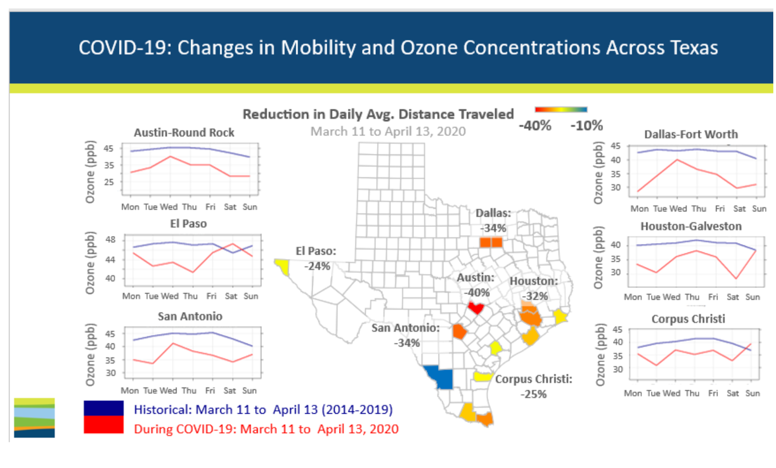
Visualization Critique
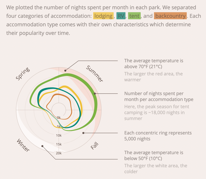
Visualization Critique
Checking in
How did it go yesterday?
How much do you feel like you remember?
Ready to keep going?
Flight data
Flight data
nycflightsSpd<-mutate(nycflights,speed = distance / air_time * 60)

nycflightsCarrSpd<-select(nycflightsSpd,year:day,carrier,flight,speed)

nycflightsCarrSpd
# A tibble: 32,735 × 6
year month day carrier flight speed
<int> <int> <int> <chr> <int> <dbl>
1 2013 6 30 VX 407 474.
2 2013 5 7 DL 329 444.
3 2013 12 8 DL 422 395.
4 2013 5 14 DL 2391 447.
5 2013 7 21 9E 3652 355.
6 2013 1 1 AA 353 319.
7 2013 12 9 WN 1428 353.
8 2013 8 13 B6 1407 285
9 2013 9 26 AA 2279 444.
10 2013 4 30 EV 4162 447.
# ℹ 32,725 more rowsFlight data
| function | process | data object |
|---|---|---|
| mutate | add speed column | nycflightsSpd |
| select | subset columns to date, carrier, flight #, and speed | nycflightsCarrSpd |
| filter | subset to flights in January | nycflightsCarrSpdJan |
| unite | combine year, month, and day into single column | nycflightsCarrSpdJanYMD |
Flight data
| function | process | data object |
|---|---|---|
| mutate | add speed column | nycflights1 |
| select | subset columns to date, carrier, flight #, and speed | nycflights2 |
| filter | subset to flights in January | nycflights3 |
| unite | combine year, month, and day into single column | nycflights4 |
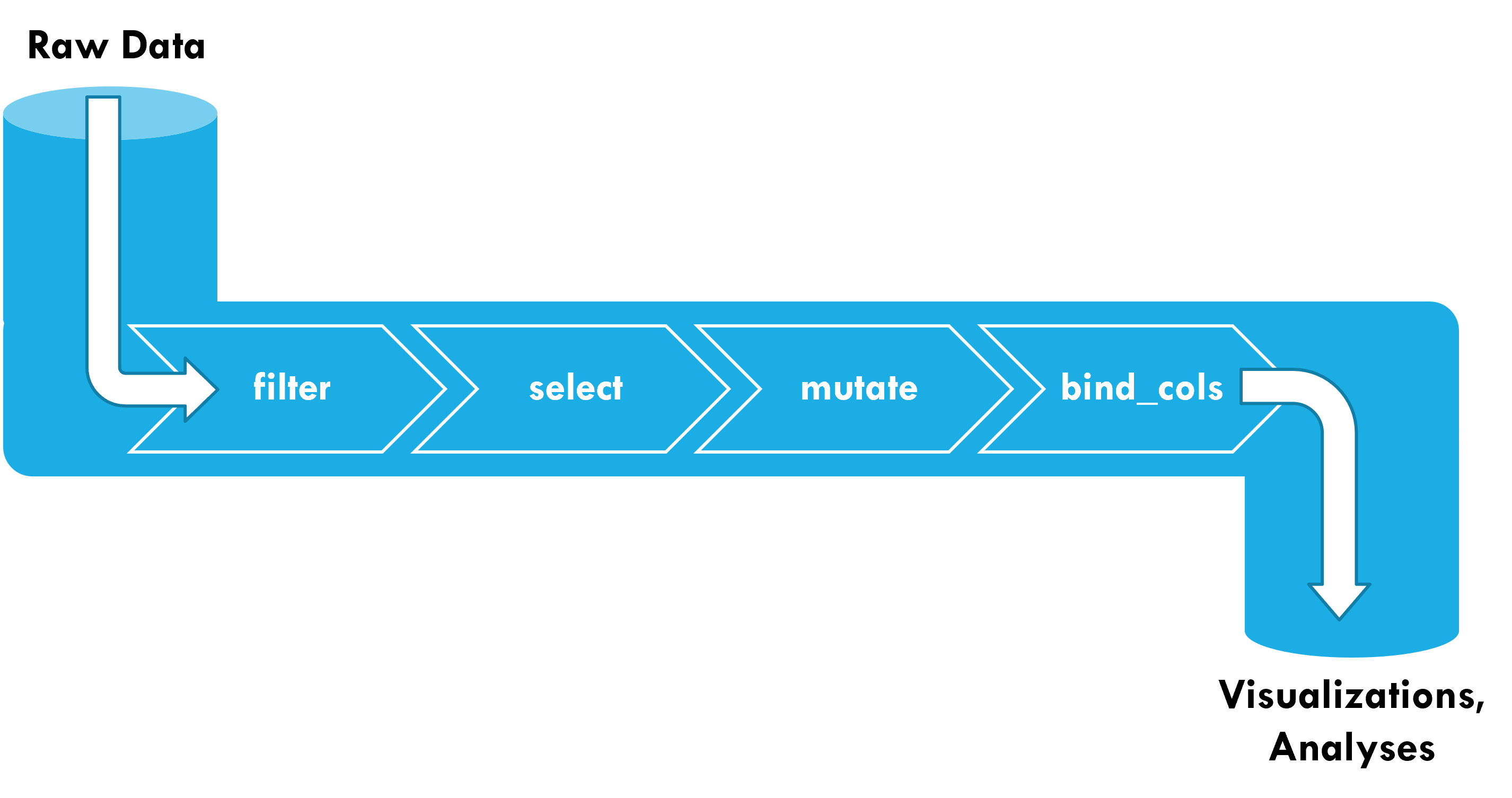
Pipes in R
The pipe operator |> allows us to combine multiple functions into a single,
nycflights |>
  mutate(speed = distance / air_time * 60) |>
  select(year:day,dep_time,carrier,flight,speed) |>
  filter(month==1) |>
  unite(col="Date",c(month,day,year),sep="/")
# A tibble: 2,610 × 5
Date dep_time carrier flight speed
<chr> <int> <chr> <int> <dbl>
1 1/1/2013 1817 AA 353 319.
2 1/23/2013 2024 EV 4412 319.
3 1/15/2013 1626 B6 369 414
4 1/17/2013 626 US 1433 311.
5 1/8/2013 902 B6 56 340.
6 1/15/2013 1947 AA 575 396.
7 1/1/2013 1454 EV 4390 363.
8 1/30/2013 1306 EV 4120 277.
9 1/4/2013 1942 B6 645 466.
10 1/8/2013 1859 AA 21 441.
# ℹ 2,600 more rowsPipelines
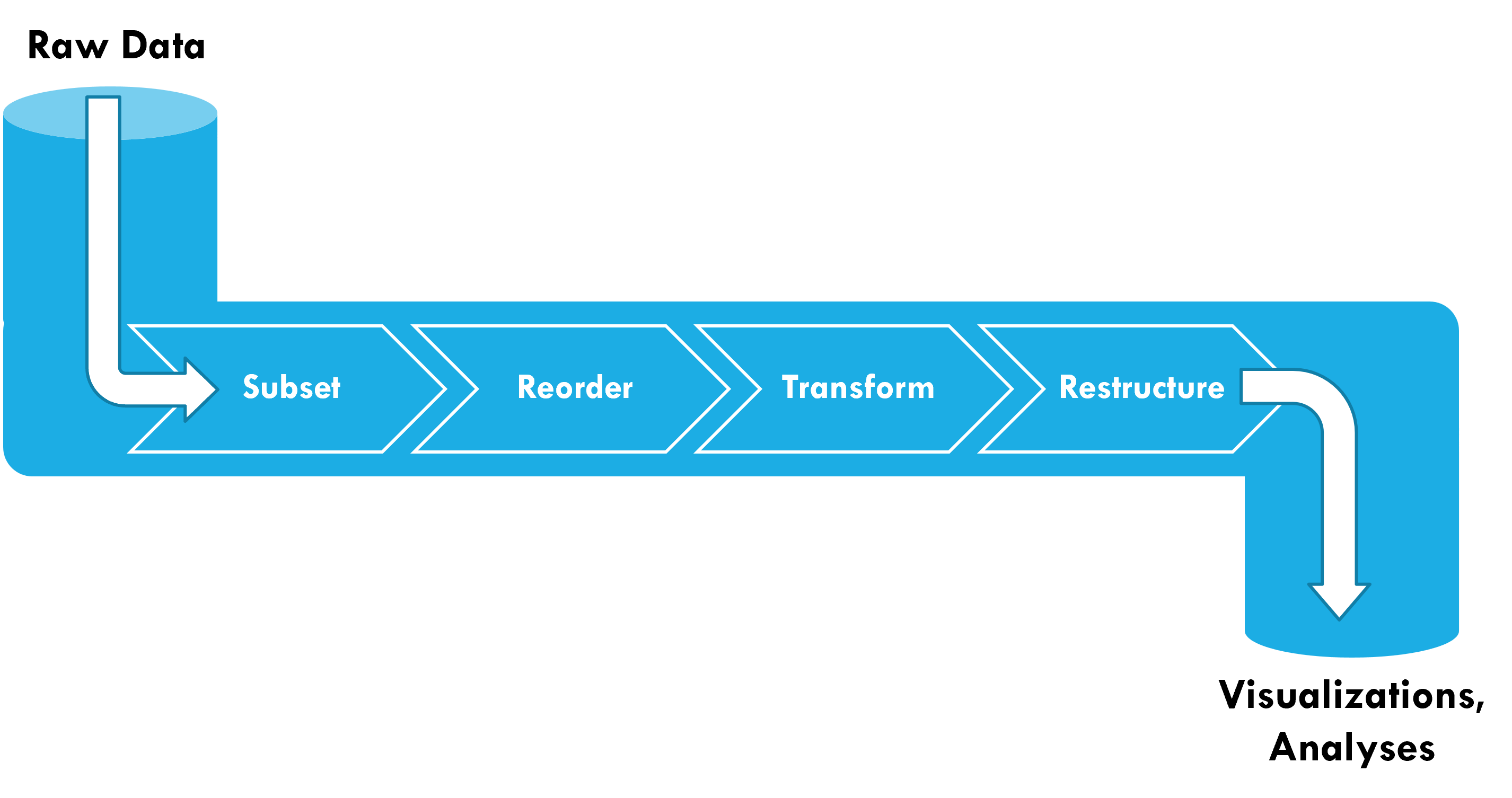
Pipelines
Pipelines start with raw data (e.g., tibble) as the input
This table is passed as the first argument to the next function (so they don’t need the data argument)
The result of a pipeline is a dataset that can be fed into visualizations and analysis
Pipes
Activity: Plumbing 101
Working in pairs or small groups, use the different functions from dplyr and tidyr to create a pipeline to wrangle raw data into the desired form
Use cheatsheets on Canvas for function descriptions
Example 1
Body mass and flipper length for penguins from Biscoe and Dream islands with a body mass over 400 grams.
Example 2
Price, number of baths, and square meters for three-bedroom homes in Sacramento.
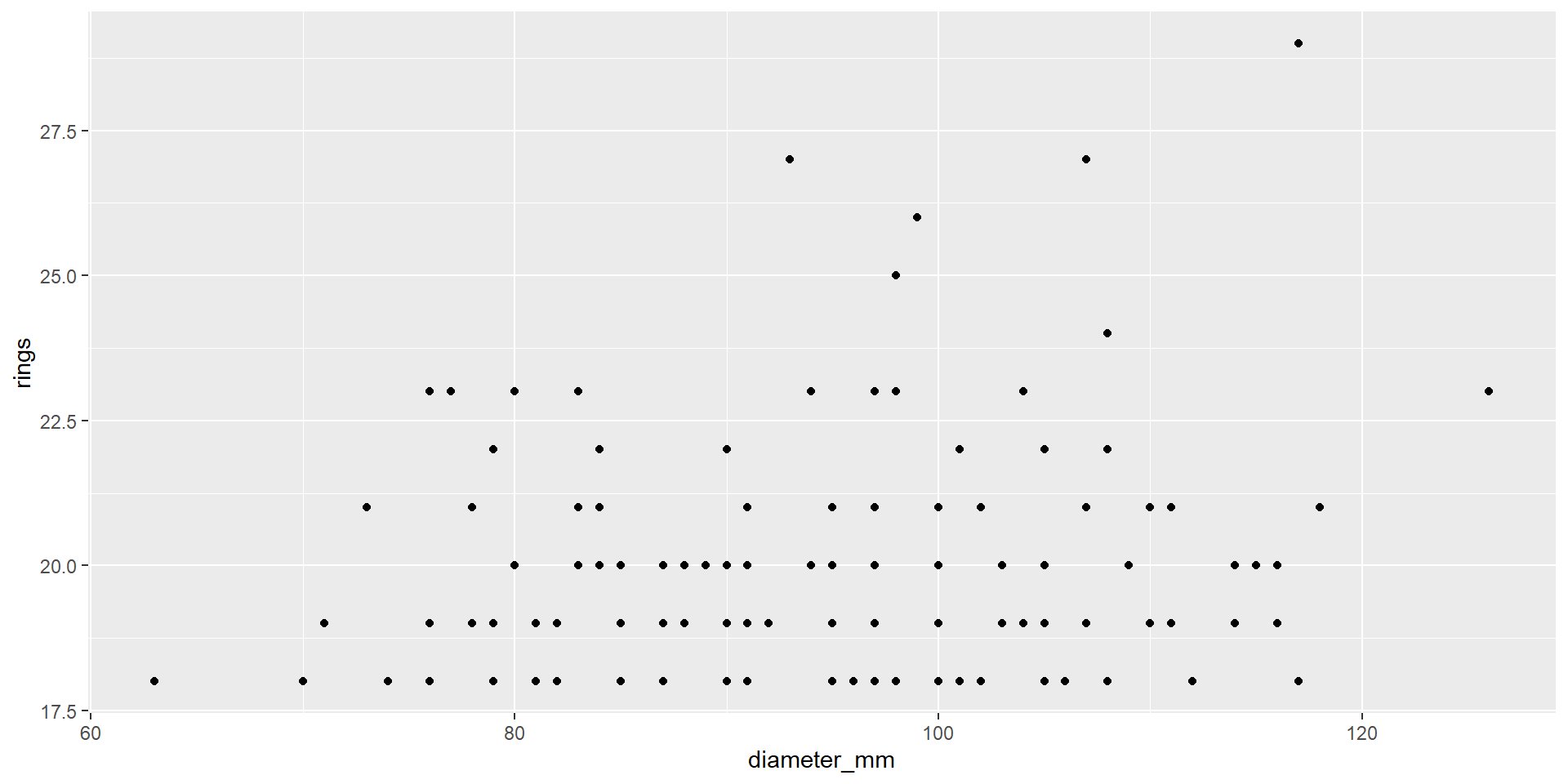
Example 3
ID Number, Diameter in mm, and number of rings on top 100 abalone by ring count.
Example 3
rawData<-read_csv("data/abalone.csv")

rawData |>
  mutate(diameter_mm=diameter * 200) |>
  select(...1,diameter_mm,rings) |>
  slice_max(order_by=rings,n=100)
# A tibble: 136 × 3
...1 diameter_mm rings
<dbl> <dbl> <dbl>
1 481 117 29
2 2109 107 27
3 2210 93 27
4 295 99 26
5 2202 98 25
6 3150 108 24
7 3281 108 24
8 314 94 23
9 315 97 23
10 502 104 23
# ℹ 126 more rowsActivity: Plumbing 101, part 2
Load the openintro package (if you don’t have it installed, install it from the command line)
We’ll be using the gss2010 dataset. Look at help to find metadata.
Using pipes, create a dataset of individuals who have attended college/university with the following variables:
hours worked per week
hours relaxing per week (assume a 7-day week)
hours not spent at work or relaxing
educational degree
attitude towards marijuana legalization
Can I use pipes with ggplot2?
Can I use pipes with ggplot2?
YES!
Can I use pipes with Base R?
Can I use pipes with Base R?
YES! (But only for functions where the first argument is a table)
Can I use pipes for modeling data?
Can I use pipes for modeling data?
YES! (But
rawData |>
  mutate(diameter_mm=diameter * 200) |>
  select(...1,diameter_mm,rings) |>
  slice_max(order_by=rings,n=100) |>
  lm(rings ~ diameter_mm, data=_) |>
  summary()
Call:
lm(formula = rings ~ diameter_mm, data = slice_max(select(mutate(rawData,
    diameter_mm = diameter * 200), ...1, diameter_mm, rings),
    order_by = rings, n = 100))

Residuals:
    Min      1Q  Median      3Q     Max
-2.3617 -1.5264 -0.5144  0.7875  8.6383

Coefficients:
            Estimate Std. Error t value Pr(>|t|)
(Intercept) 17.56936    1.41959  12.376   <2e-16 ***
diameter_mm  0.02387    0.01477   1.616    0.108
---
Signif. codes:  0 '***' 0.001 '**' 0.01 '*' 0.05 '.' 0.1 ' ' 1

Residual standard error: 2.074 on 134 degrees of freedom
Multiple R-squared:  0.01912,   Adjusted R-squared:  0.0118
F-statistic: 2.612 on 1 and 134 DF,  p-value: 0.1084
Next week
Visualizing more relationships
Fine controls with ggplot2
Time series data