Environmental Data Analysis & Visualization
Does anybody really know what time it is?
Warm-up exercise
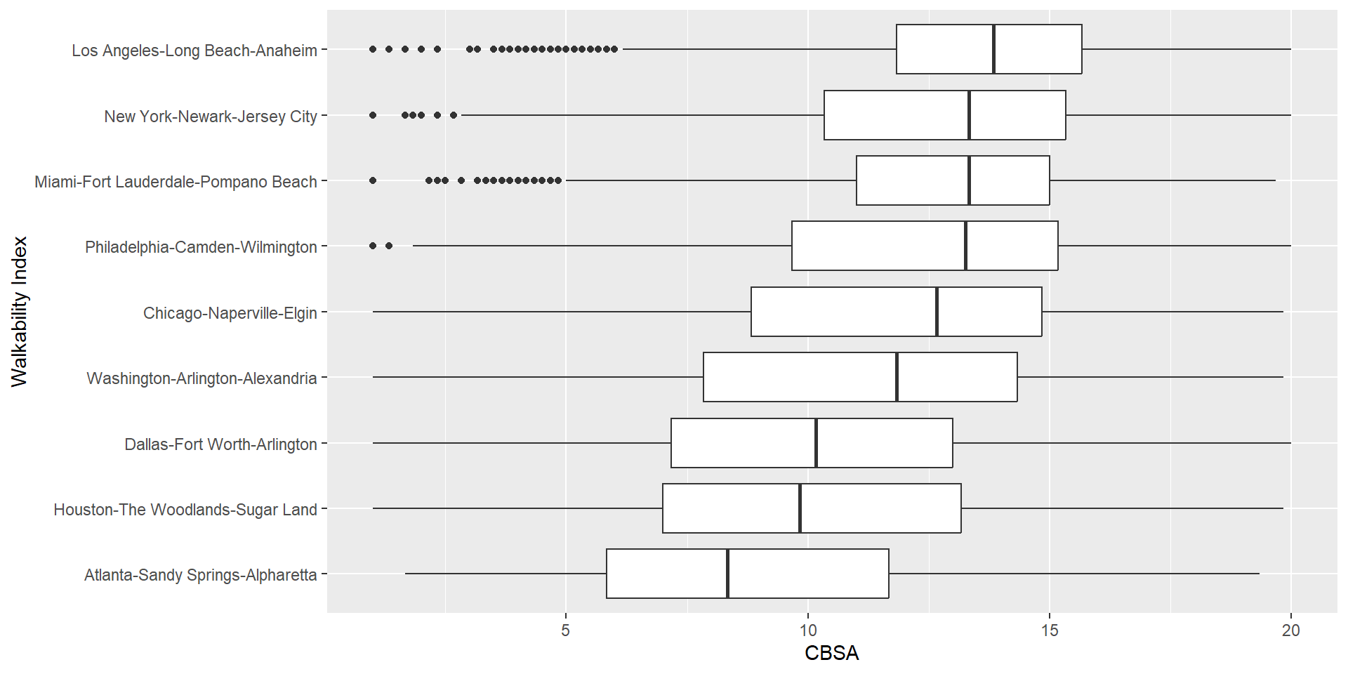
Create a new file system and Quarto document for this lecture. Download the walkability.csv dataset. Using pipes, create a dataset of with the following variables:
Core-Based Statistical Area (CBSA) name (excluding the state)
Population (only above 5 million)
National Walkability Index
Show the distribution of walkability index scores for all CBSAs in this new dataset
Warm-up exercise
<- read_csv ("data/walkability.csv" ) %>% select (CBSA_Name,CBSA_POP,NatWalkInd) %>% separate (CBSA_Name,into= c ("cities" ,"states" ),sep= "," ,extra= "drop" ) %>% filter (CBSA_POP> 5000000 ) %>% ggplot (aes (x= reorder (cities,NatWalkInd,median),y= NatWalkInd)) + geom_boxplot () + coord_flip () + labs (x= "Walkability Index" ,y= "CBSA" )
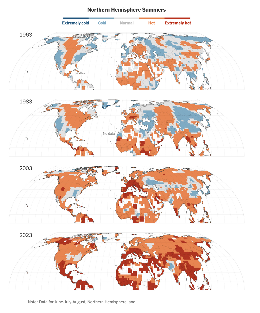
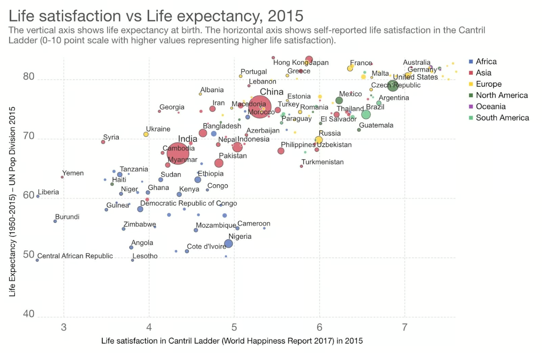
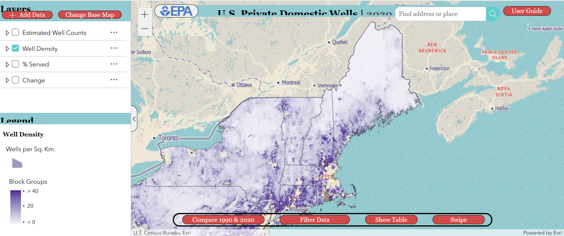
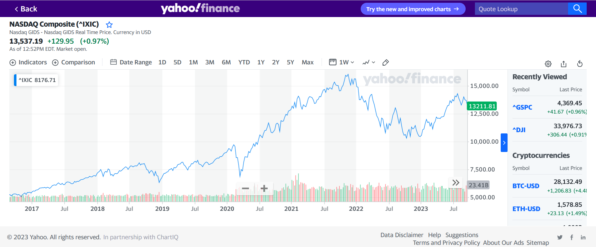
Visualization critique
https://experience.arcgis.com/experience/be9006c30a2148f595693066441fb8eb/page/Map/
When does “when” matter?
Time: what is it?
R can store time as character values.
"2023-10-19"
"10/19/2023"
"17:05:00"
Time: what is it?
It can also store some kinds of time data as numbers:
Time: what is it?
Time by itself isn’t something that varies in a meaningful way.
Time has a defined order, but you can’t really count time, nor can you really treat it like a number.
Time: what is it?
R can also recognize time as particular objects like date and date-time objects. For example:
#give today's date as a date object today ()#give the precise time as a date-time object now ()
[1] "2023-10-20 12:51:43 EDT"
Handling time data
The lubridate package lets us convert between other values and time objects.
Handling time data
#storing the date as a character value <- "2023-10-19"
Handling time data
# converting the date to a date object ymd (todaysDate)
Visualizing time data
NASDAQ Composite data
<- read_csv ("data/nasdaq.csv" )
# A tibble: 65 × 7
   Date        Open   High    Low  Close `Adj Close`     Volume
   <chr>      <dbl>  <dbl>  <dbl>  <dbl>       <dbl>      <dbl>
 1 7/18/2023 14212. 14397. 14176. 14354.      14354. 4824070000
 2 7/19/2023 14399. 14447. 14317. 14358.      14358. 5112420000
 3 7/20/2023 14273. 14310. 14031. 14063.      14063. 5128020000
 4 7/21/2023 14148. 14179. 14020. 14033.      14033. 5254180000
 5 7/24/2023 14082. 14110. 13997. 14059.      14059. 4083070000
 6 7/25/2023 14093. 14202. 14093. 14145.      14145. 3812470000
 7 7/26/2023 14124. 14187. 14042. 14127.      14127. 4322000000
 8 7/27/2023 14319. 14360. 14007. 14050.      14050. 5115840000
 9 7/28/2023 14200. 14344. 14188. 14317.      14317. 4453520000
10 7/31/2023 14338. 14371. 14293. 14346.      14346. 4934440000
# ℹ 55 more rows
Visualizing time data
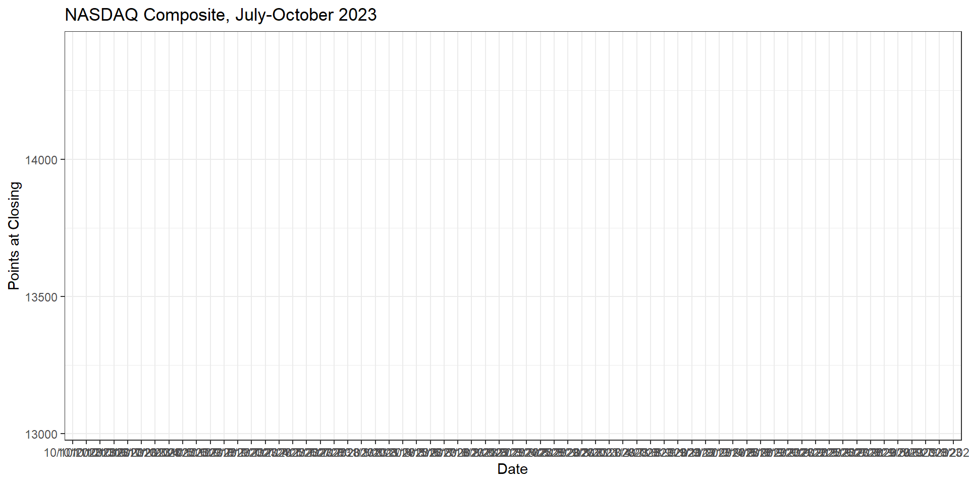
ggplot (nasdaq,aes (x= Date,y= Open)) + geom_line (color= "darkblue" ) + labs (x= "Date" ,y= "Points at Closing" ,title= "NASDAQ Composite, July-October 2023" ) + theme_bw ()
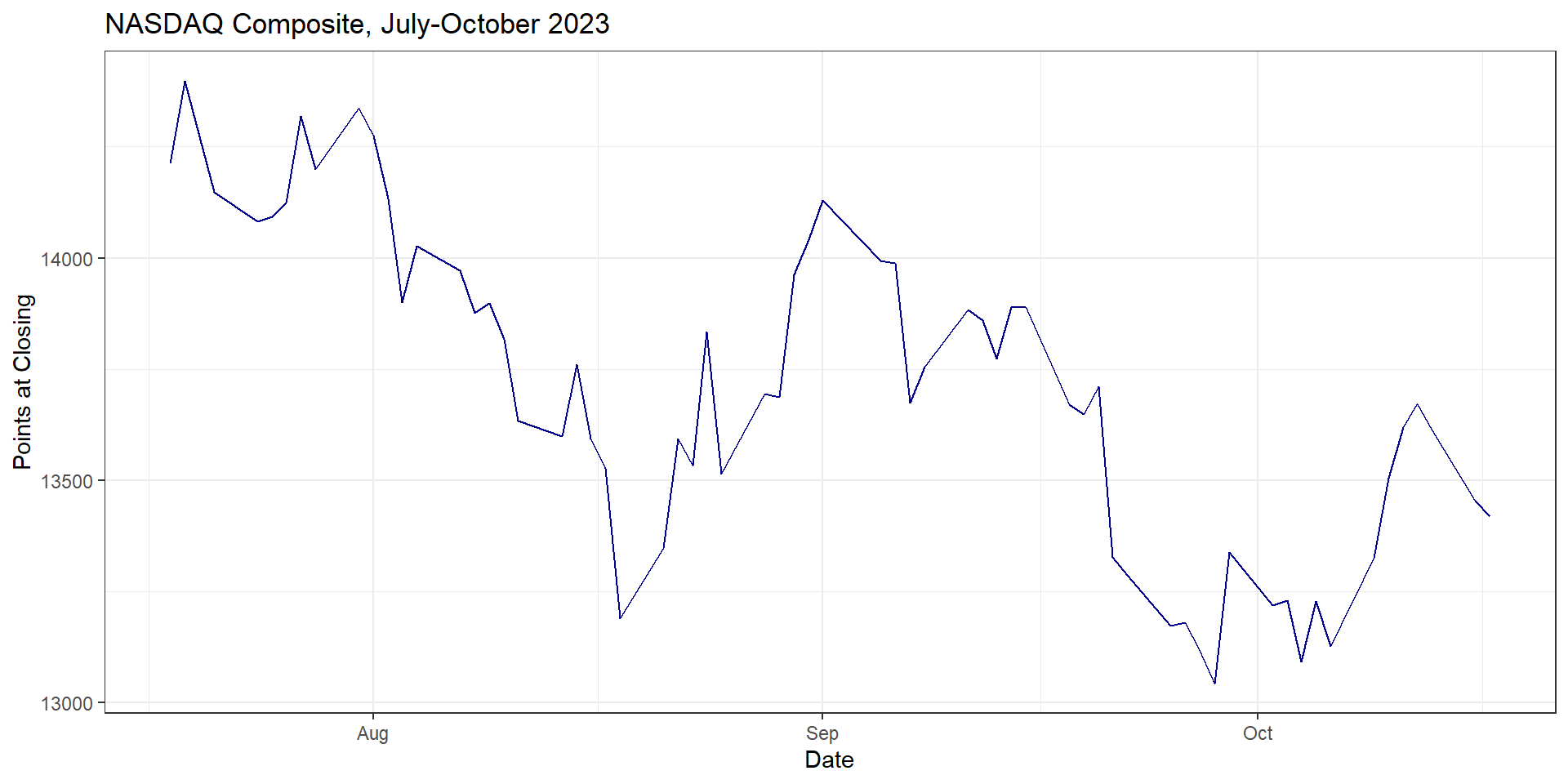
Visualizing time data
ggplot (nasdaq,aes (x= mdy (Date),y= Open)) + geom_line (color= "darkblue" ) + labs (x= "Date" ,y= "Points at Closing" ,title= "NASDAQ Composite, July-October 2023" ) + theme_bw ()
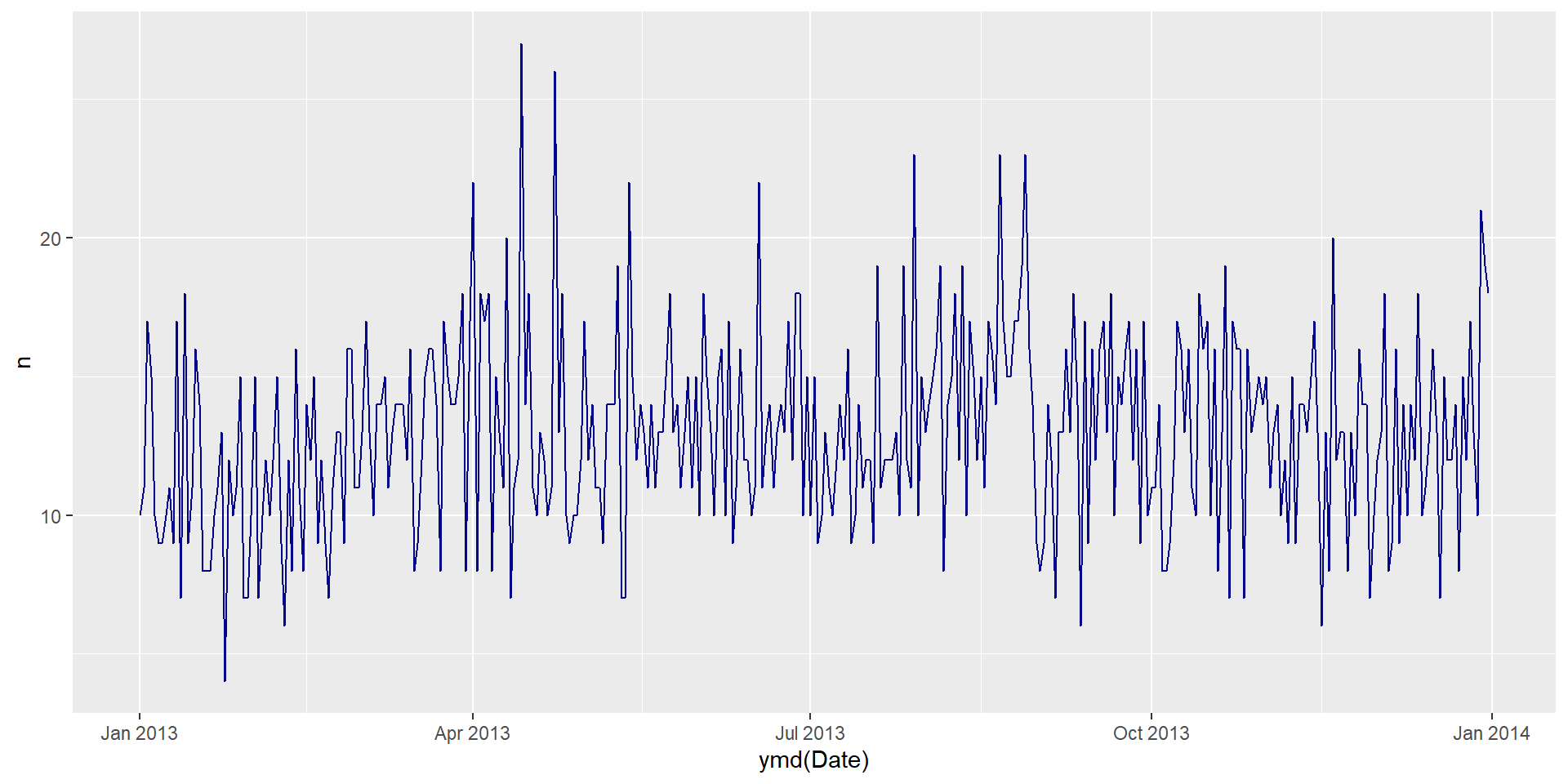
Activity: Visualizing time data
Load the openintro package to access the nycflights data
Create a pipe that
subsets the data to Delta Airlines (DL) flights only
combines the year, month, and day into a single date column
convert to a table of counts using the count function
Plot this new data as a line graph using geom_line.
Activity: Visualizing time data
<- nycflights|> filter (carrier== "DL" ) |> unite (col= "Date" ,year,month,day,sep= "-" ,na.rm = TRUE ) |> count (Date)|> ggplot (aes (x= ymd (Date),y= n)) + geom_line (color= "darkblue" )