Environmental Data Analysis and Visualization
The Data Goes On and On (and On and On…)
Warm-up exercise
Download the Lecture16data.zip file and extract the files into your working directory.
Load in the denverGrocery and statistical_neighborhoods shapefile as sf objects
Plot these using geom_sf and color the stores according to type
Warm-up exercise
library(sf)
library(tidyverse)
library(sf)
grocStores<-st_read("data/denverGrocery.shp",quiet=TRUE)
neighborhoods<-st_read("data/statistical_neighborhoods.shp",quiet=TRUE)
ggplot()+
  geom_sf(data=neighborhoods) +
  geom_sf(data=grocStores,aes(color=STORE_TYPE)) +
  theme_minimal() +
  labs(x="Longitude",y="Latitude",color="Store Type",title="Food Stores in Denver")
Warm-up exercise
![]()
Dataset of the day
Massachusetts Community Health Data
![]()
Mass.gov
Errata
library(tidyverse)
library(sf)

data<-read_csv("data/whereEat2.csv")
data2<-data %>% filter(Longitude < -70) %>% filter(Latitude > 40)

boston<-st_read("data/City_of_Boston_Boundary.shp",quiet=TRUE)
eatSpat<-st_as_sf(data2,coords=c("Longitude","Latitude"))
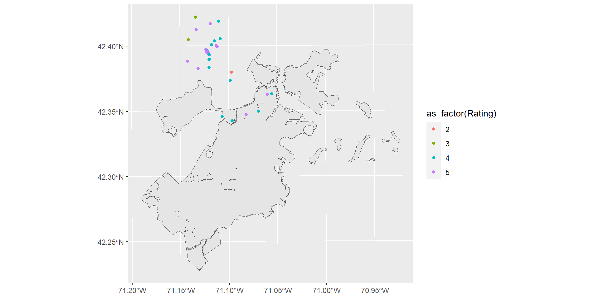
Errata
st_crs(eatSpat)<-4326
eatSpat2<-st_transform(eatSpat,st_crs(boston))

ggplot()+
  geom_sf(data=boston) +
  geom_sf(data=eatSpat2,aes(color=as_factor(Rating)))
![]()
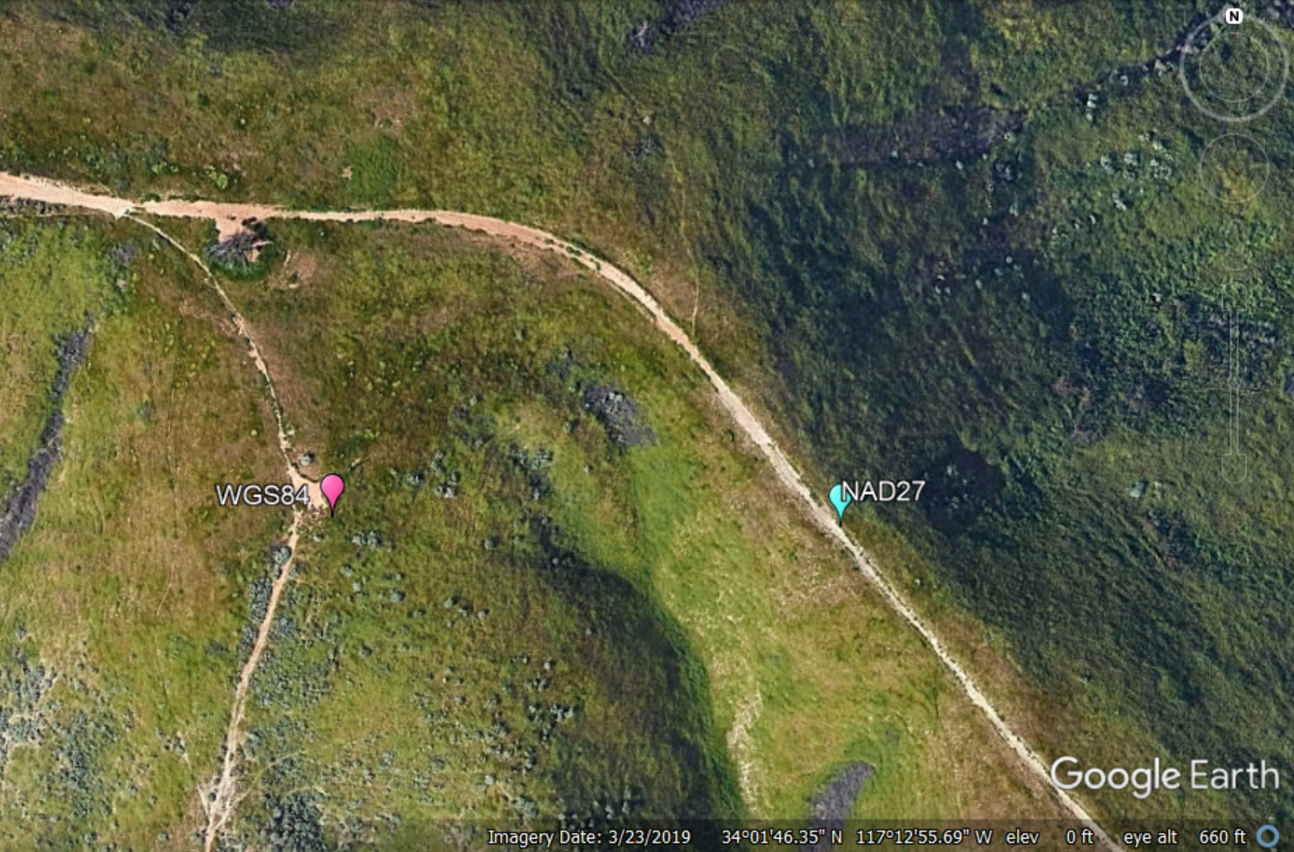
Why does the CRS matter?
Coordinates from one CRS may look similar but be in quite different locations
![]()
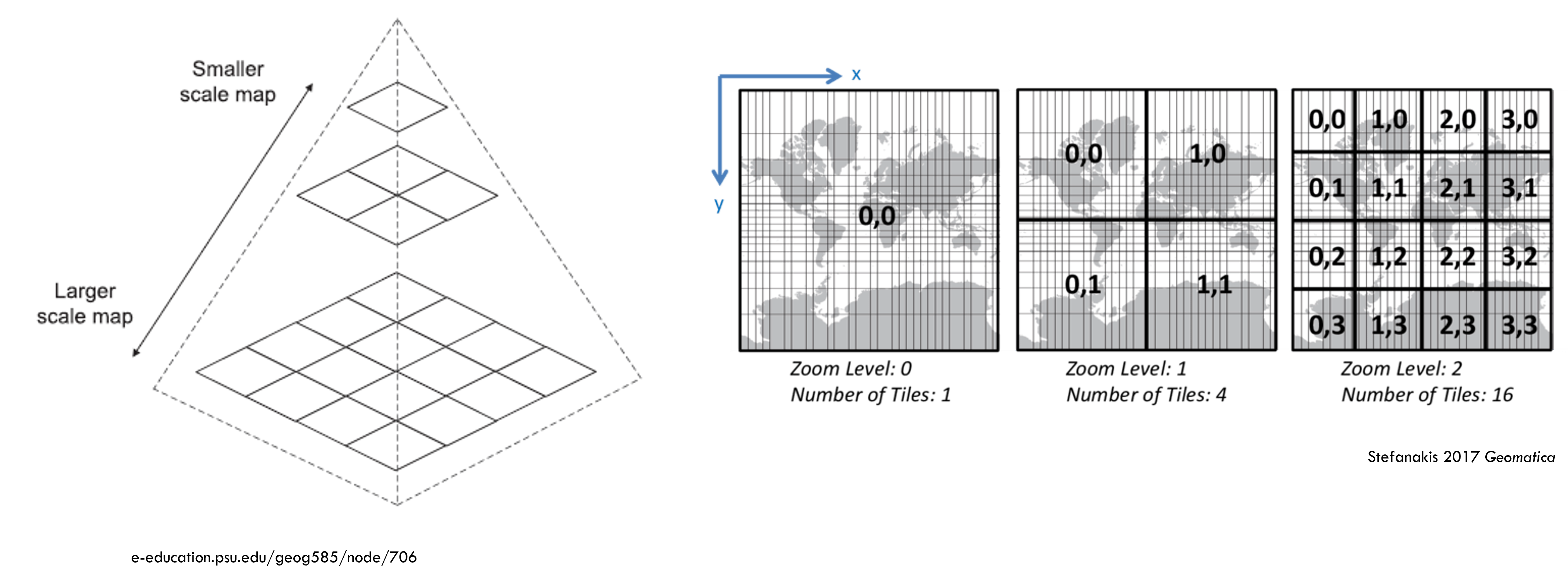
Basemaps
![]()
Google Maps
Basemaps
![]()
Basemaps with maptiles
library(terra)
library(tidyterra)
library(maptiles)
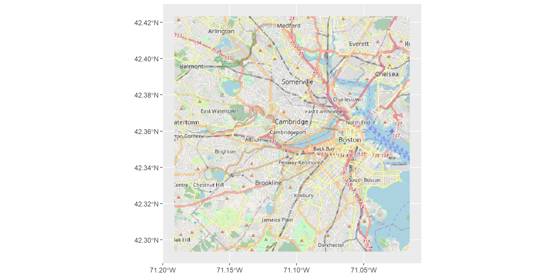
Basemaps with maptiles
base<-get_tiles(eatSpat)

ggplot() +
    geom_spatraster_rgb(data=base)
![]()
Basemaps with maptiles
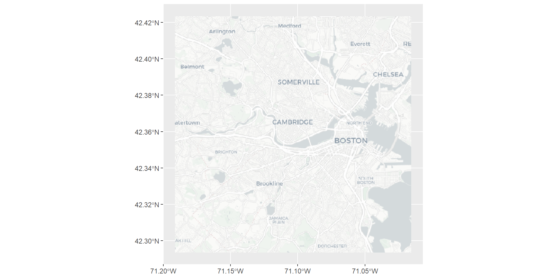
base<-get_tiles(eatSpat,provider="CartoDB.Positron")

ggplot() +
    geom_spatraster_rgb(data=base)
![]()
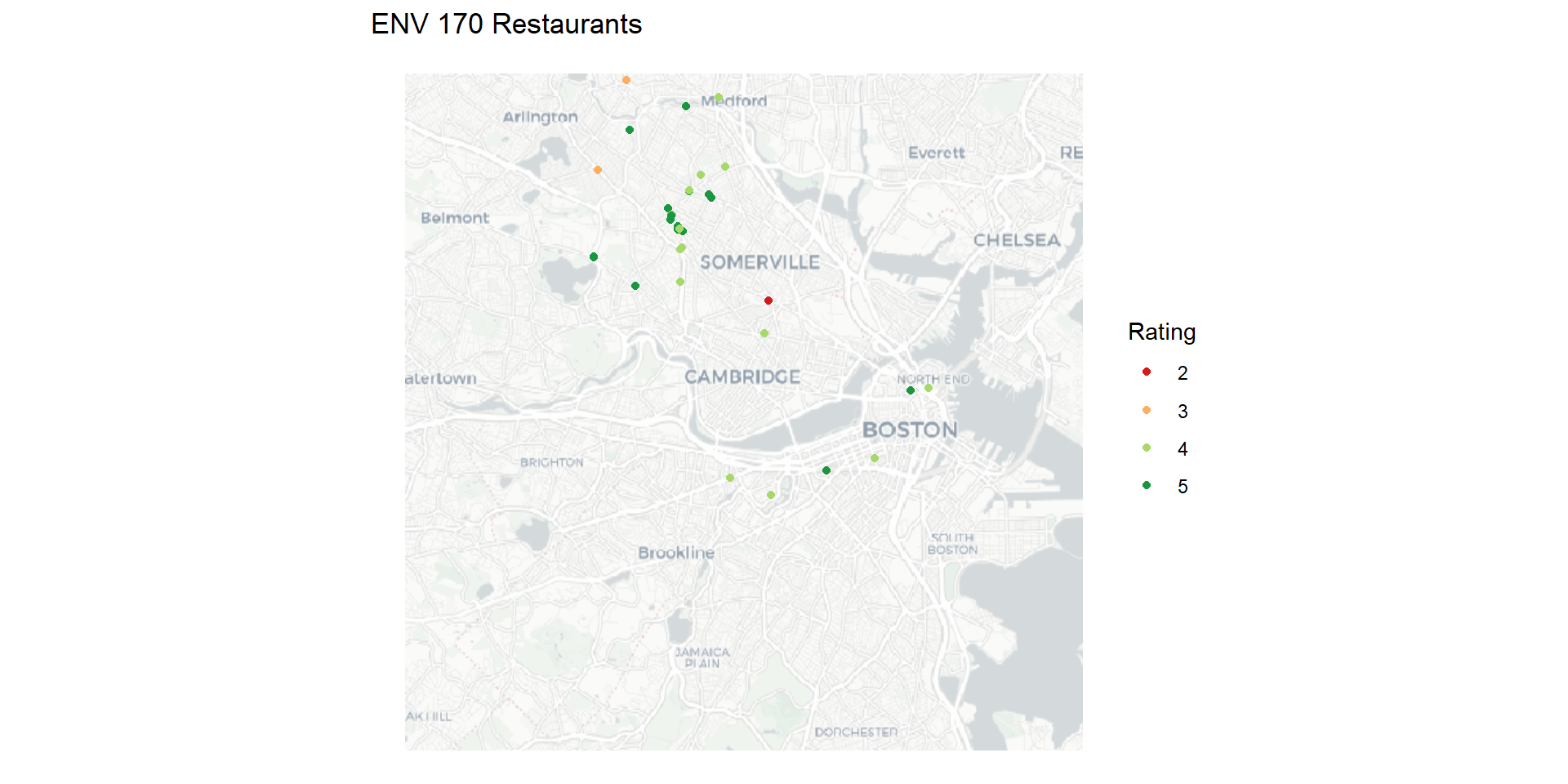
Basemaps with maptiles
ggplot() +
    geom_spatraster_rgb(data=base) +
  geom_sf(data=eatSpat,aes(color=as_factor(Rating))) +
  labs(title="ENV 170 Restaurants",color="Rating") +
  theme_void() +
  scale_color_brewer(palette="RdYlGn")
![]()
Interactive maps in R with leaflet
Leaflet is used in many web-mapping applications, and can be used in R via the leaflet package.
![]()
Interactive maps in R with leaflet
leaflet() %>%
  setView(lng = -71.11345, lat = 42.38945, zoom = 12) %>%
  addTiles()
Interactive maps in R with leaflet
leaflet() %>%
  setView(lng = -71.11345, lat = 42.38945, zoom = 12) %>%
  addProviderTiles(providers$CartoDB.Positron)
Interactive maps in R with leaflet
leaflet(eatSpat) %>%
  addProviderTiles(providers$CartoDB.Positron) %>%
  addCircleMarkers(radius=2,color="blue",label=~Name)
Activity: Interactive maps
Using the Denver food store data, make a map of the grocery stores using either maptiles or leaflet
Modify the background by tile provider to improve the visibility of the data or it’s ability to catch the eye.
Activity: Interactive maps
maptiles
base<-get_tiles(eatSpat,provider="CartoDB.Positron")

ggplot() +
    geom_spatraster_rgb(data=base)
leaflet
leaflet(eatSpat) %>%
  addProviderTiles(providers$CartoDB.Positron) %>%
  addCircleMarkers(radius=2,color="blue",label=~Name)
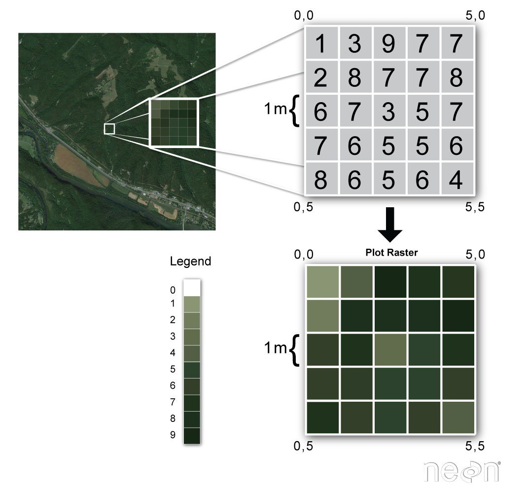
Raster data
Rasters are used to represent spatial information that has a continuous distribution.
![]()
datacarpentry.org
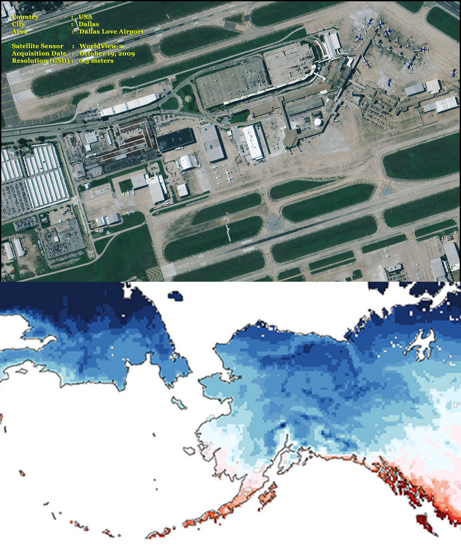
What kind of data comes as a raster?
Satellite imagery
Climate model outputs
Oceanographic data
Elevation models
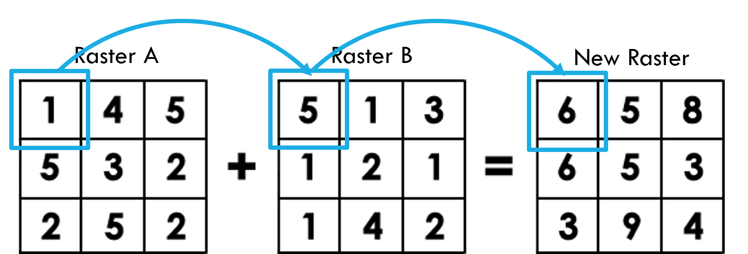
Raster algebra
Raster cells contain values that can be combined with cell values of other rasters at the same locations to produce a new raster
![]()
Mapping out the rest of the week