3  Manipulating rasters

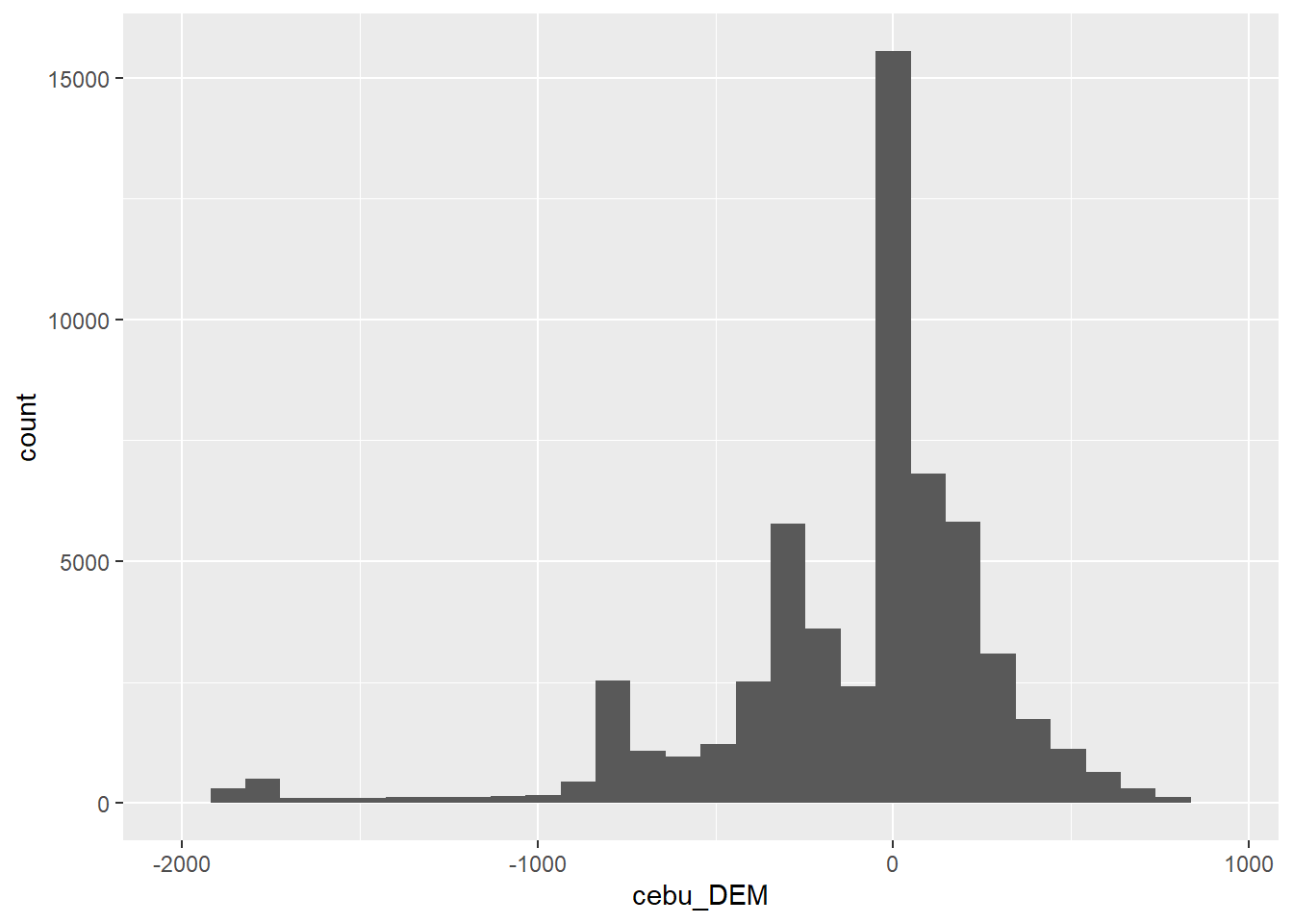
Warning: package 'terra' was built under R version 4.4.2

Warning: package 'tidyterra' was built under R version 4.4.2

As mentioned earlier, we can get all of the values in our raster by using the values function. This can be useful if we’re interested in visualizing the data in another way. For example, as a histogram:

elevations<-values(cebuDEM)
ggplot(data=elevations,aes(cebu_DEM))+
  geom_histogram()

`stat_bin()` using `bins = 30`. Pick better value with `binwidth`.

Notice here how the variable mapped on to x was cebu_DEM. This is the name of the file that the data came from rather than the object we stored it in. This is the default label used by terra when data is read in from a file.

What if we just wanted a value from a single location? We can use the extract function to get at these, using a set of coordinates stored in a tibble:

x<-c(123.58)
y<-c(10.13)
xy<-tibble(x,y)
pointData<-extract(cebuDEM, xy)
pointData

  ID cebu_DEM
1  1      169

Try it yourself!

Let’s say we wanted to get a random sample of 50 elevations from the Turkana and Cebu elevation data. How would you go about it? Can you plot these as a histogram?

Raster algebra

Raster algebra is the task of modifying values . You could think of this as akin to the mutate function. For example, let’s say we wanted to convert our elevation data, currently in feet above sea level, to meters. The conversion from meters to feet is:

\[ f \times 3.28 \]

To apply this across our raster, we simply multiply it by 3.28.

#convert m to feet
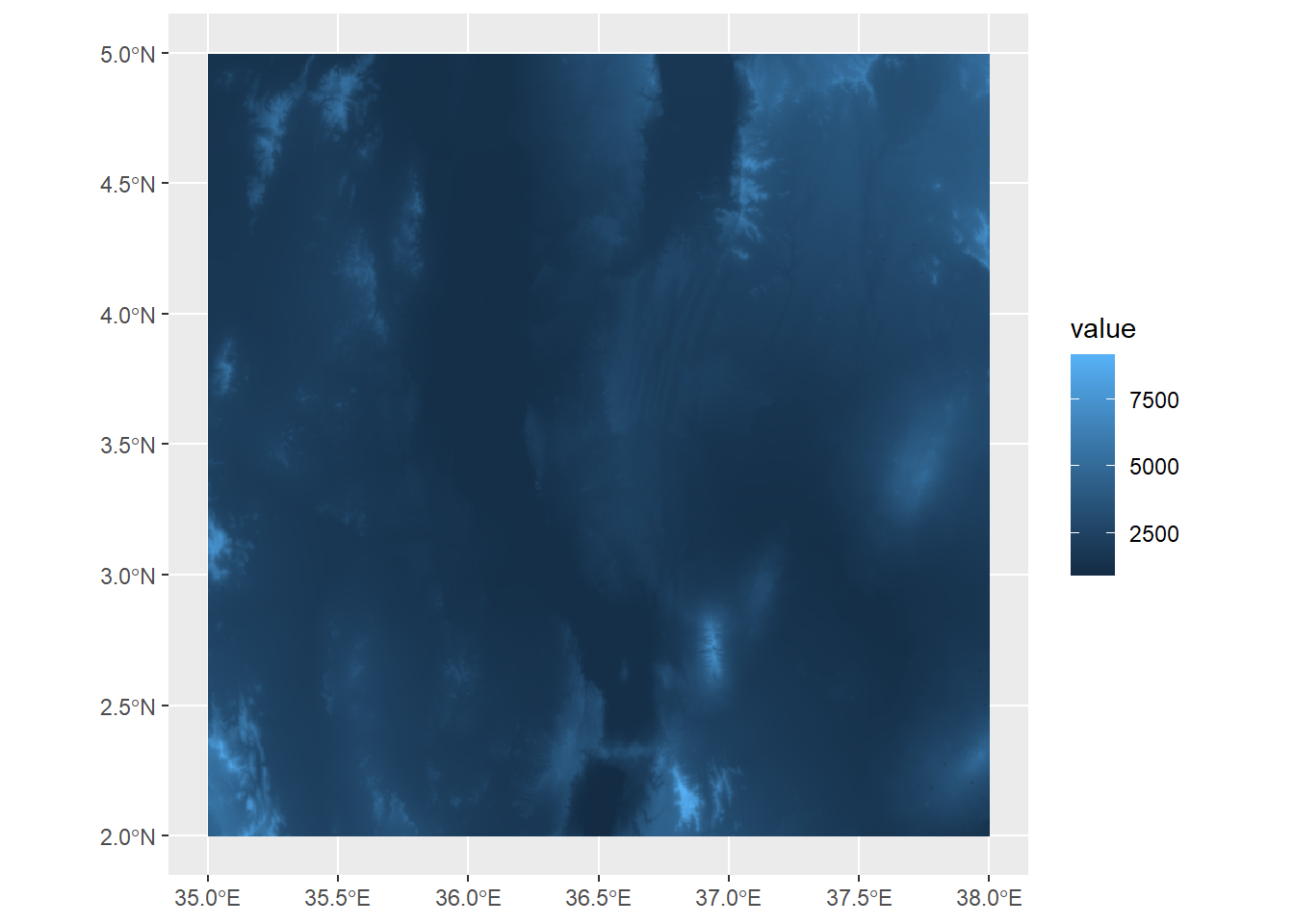
turkanaDEM_ft<-turkanaDEM*3.28
ggplot()+
  geom_spatraster(data=turkanaDEM_ft)

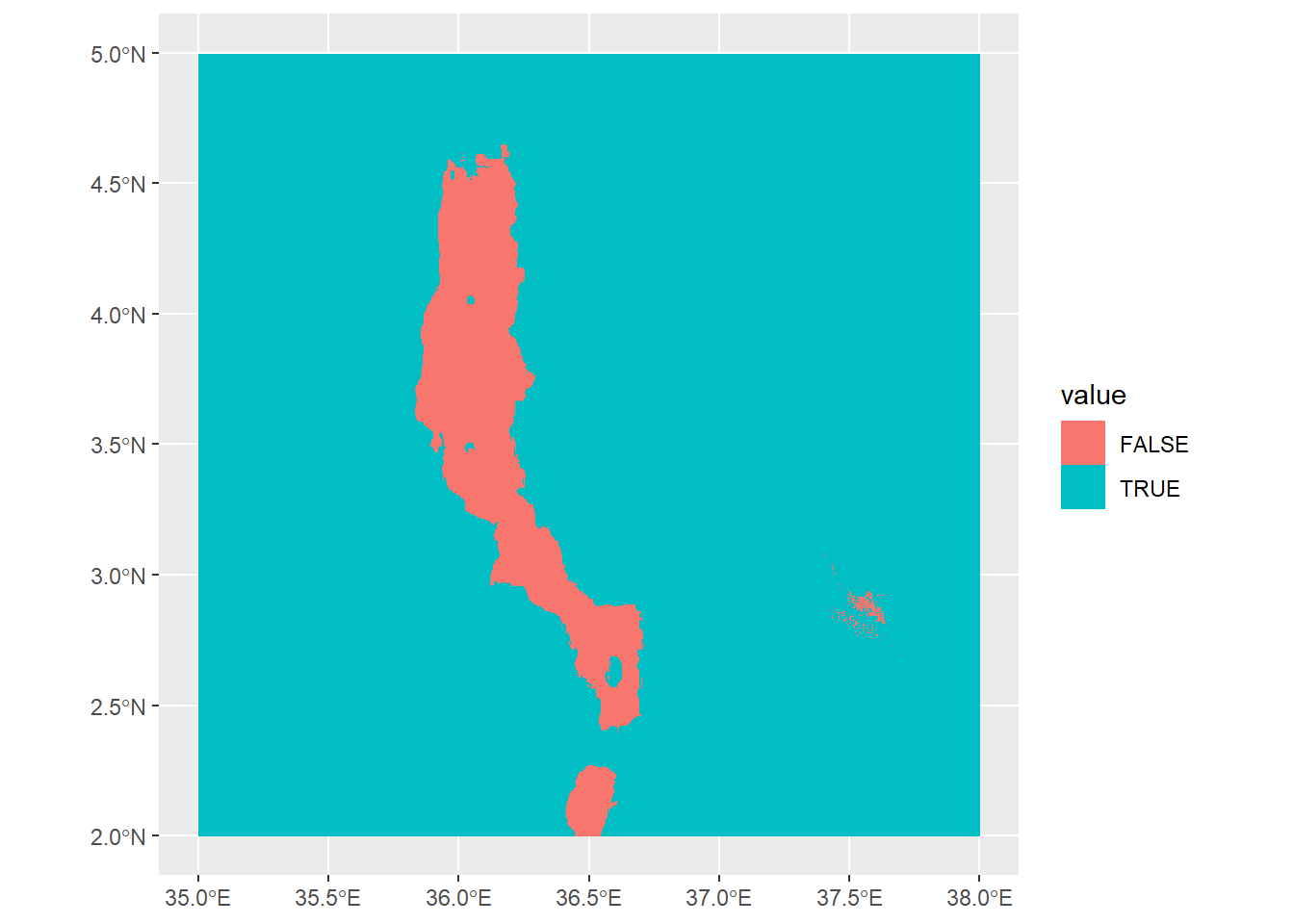
The surface of Lake Turkana is about 1200 feet above sea level. We could just get those cells above the lake level using the same kind of algebra.

turkanaLand<-turkanaDEM_ft>1200
ggplot()+
  geom_spatraster(data=turkanaLand)

Here, the raster returned to us is a Boolean (true/false) raster.

We can also use raster algebra on more than one raster. For example, let’s say we wanted to sum the rainfall for the first four months in the rainfall data. We can use our turkanaRain4 data from earlier and sum the values in the four layers:

#convert m to feet
turkanaRain_JanApr<-sum(turkanaRain4)
turkanaRain_JanApr

class       : SpatRaster 
dimensions  : 72, 72, 1  (nrow, ncol, nlyr)
resolution  : 0.04166667, 0.04166667  (x, y)
extent      : 35, 38, 2, 5  (xmin, xmax, ymin, ymax)
coord. ref. : lon/lat WGS 84 (EPSG:4326) 
source(s)   : memory
name        :   sum 
min value   :  97.1 
max value   : 414.9 

As you can see, this creates a new raster based on the sum of the four layers in the dataset.

Try it yourself!

Try seeing if you can take the mean of the first twelve layers of the rainfall data and convert it into inches.