A model is something that represents some aspect of the real world by way of an analogy. A model train, for example, can represent aspects of a real locomotive like wheels and car couplings. Computer simulations are a class of models that can be used to represent all kinds of phenomena, from solar systems to human organs.
All models share an important quality: they are all imperfect representations of the real phenomenon. However, despite their imperfections, they are often used to help us better understand the world around us. There is famous quote often attributed to the statistician George Box that sums up this idea:
“All models are wrong, but some models are useful.”
This lab will deal with how to use linear models for predicting relationships between variables.
A motivating example
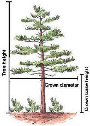
Let’s say that the city of Charlotte, NC wants to protect critical habitats in its urban forests. A recent study has shown that the endangered Carolina northern flying squirrel has a preference for Willow Oak trees above a height of 25 meters. The city parks department works with local volunteers to identify these trees; however, taking accurate height measurements can be difficult and time-consuming. They would like to find an easier way to estimate height, so they turn to you, the trusty data scientist, to try and answer this question.
The question is one of prediction: can we use the relationship between tree height and some other variable(s) in order to predict tree height.
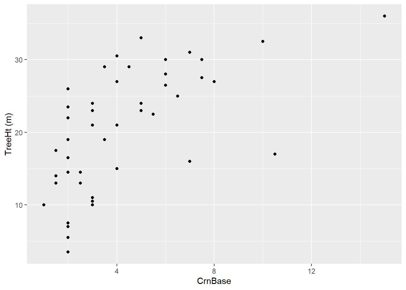
What we’d like to know is whether a linear relationship exists between crown base height and tree height. By linear, we mean that an increase of some increment in one variable (crown base height) will result in an increase in the variable of interest (tree height). Let’s see what the relationship between our variables looks like visually:
One thing to notice about the code here. First, notice that CrnBase is not surrounded by backticks, while TreeHt (m) has them. The reason is that CrnBase doesn’t have any non-standard characters like whitespace or parentheses, so the read_csv function didn’t add them.
OK, so what do we see here? Well, there does seem to be an increase, but it isn’t very strong. We can assess this strength by doing a correlation test:
    Pearson's product-moment correlation

data:  treeDataNC$CrnBase and treeDataNC$`TreeHt (m)`
t = 5.3424, df = 47, p-value = 2.62e-06
alternative hypothesis: true correlation is not equal to 0
95 percent confidence interval:
 0.4031591 0.7638432
sample estimates:
      cor
0.6146721
The cor value is 0.61, which suggests a positive relationship, but it isn’t especially strong. The p-value is very low, though, so this indicates we can reject the idea there isn’t a relationship. Of course, we didn’t check to see whether the data are normally distributed. We can use shapiro.test to do that:
    Shapiro-Wilk normality test

data:  treeDataNC$`TreeHt (m)`
W = 0.96854, p-value = 0.2117
shapiro.test(treeDataNC$CrnBase)
    Shapiro-Wilk normality test

data:  treeDataNC$CrnBase
W = 0.84429, p-value = 1.293e-05
Remembering back to last week, a p-value greater than our cut-off threshold (0.05) tells us that we can’t reject the null hypothesis that the data are normally distributed. This is true for tree height, but not so for the crown base height. So we should probably run our correlation test again, but this time using the Spearman method:
    Spearman's rank correlation rho

data:  treeDataNC$CrnBase and treeDataNC$`TreeHt (m)`
S = 6156.7, p-value = 5.37e-08
alternative hypothesis: true rho is not equal to 0
sample estimates:
      rho
0.6858807
The result is pretty similar: we can reject the idea that there is no relationship, and the data indicate a positive relationship. The rho value is a little improved, but not by a lot.
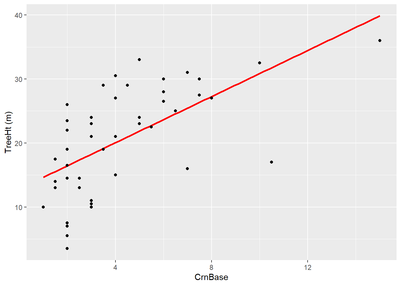
Given the existence of a relationship, we could ask: how well can we predict tree height from crown base height? A linear model can help us to estimate this. If you think back to our scatter plot, what a linear model does is draw a straight line through the data that minimizes the distance to all of the points.
`geom_smooth()` using formula = 'y ~ x'
If we find that the line fits the data well, which would be indicated by how closely the data fall along it, then we can use the line to provide us with predictions about data we have not observed. For example, looking at the plot above, the linear model would predict that a tree with a crown base height of 10 meters would have a total height of about 31 meters. Of course, the value of this prediction depends on how well the model fits the data.
To create our model, we’ll use the lm, or linear model, function:
What have we done here? What this code does is asks R to conduct a linear regression on these two variables and save it as a linear model object called treeModel. At a minimum, lm needs an argument that comes in the form of a formula:
y~x
Where y is the response variable (tree height) and x is a predictor (crown base height). If we just want to use column names like we have here, we also have to supply a data argument, which in this case is the treeDataNC tibble. We could get the same result without this argument by referring to the columns using the $ operator:
So now our model is stored as treeModel. We can get a quick look at the results by using the summary function:
summary(treeModel1)
Call:
lm(formula = treeDataNC$`TreeHt (m)` ~ treeDataNC$CrnBase)

Residuals:
     Min       1Q   Median       3Q      Max
-14.7496  -4.3383   0.9595   5.5553  11.1581

Coefficients:
                   Estimate Std. Error t value Pr(>|t|)
(Intercept)         12.8348     1.7161   7.479 1.54e-09 ***
treeDataNC$CrnBase   1.8014     0.3372   5.342 2.62e-06 ***
---
Signif. codes:  0 '***' 0.001 '**' 0.01 '*' 0.05 '.' 0.1 ' ' 1

Residual standard error: 6.591 on 47 degrees of freedom
Multiple R-squared:  0.3778,    Adjusted R-squared:  0.3646
F-statistic: 28.54 on 1 and 47 DF,  p-value: 2.62e-06
There’s a few different pieces of information here, let’s go through some of the most relevant
Residuals: Residuals are how far the real data deviate
Coefficients: These are indicating the relative increments th
R-squared: These are measures of the proportion of variance in the response variable explained by the predictor. A value of 1 would indicate a perfect match.
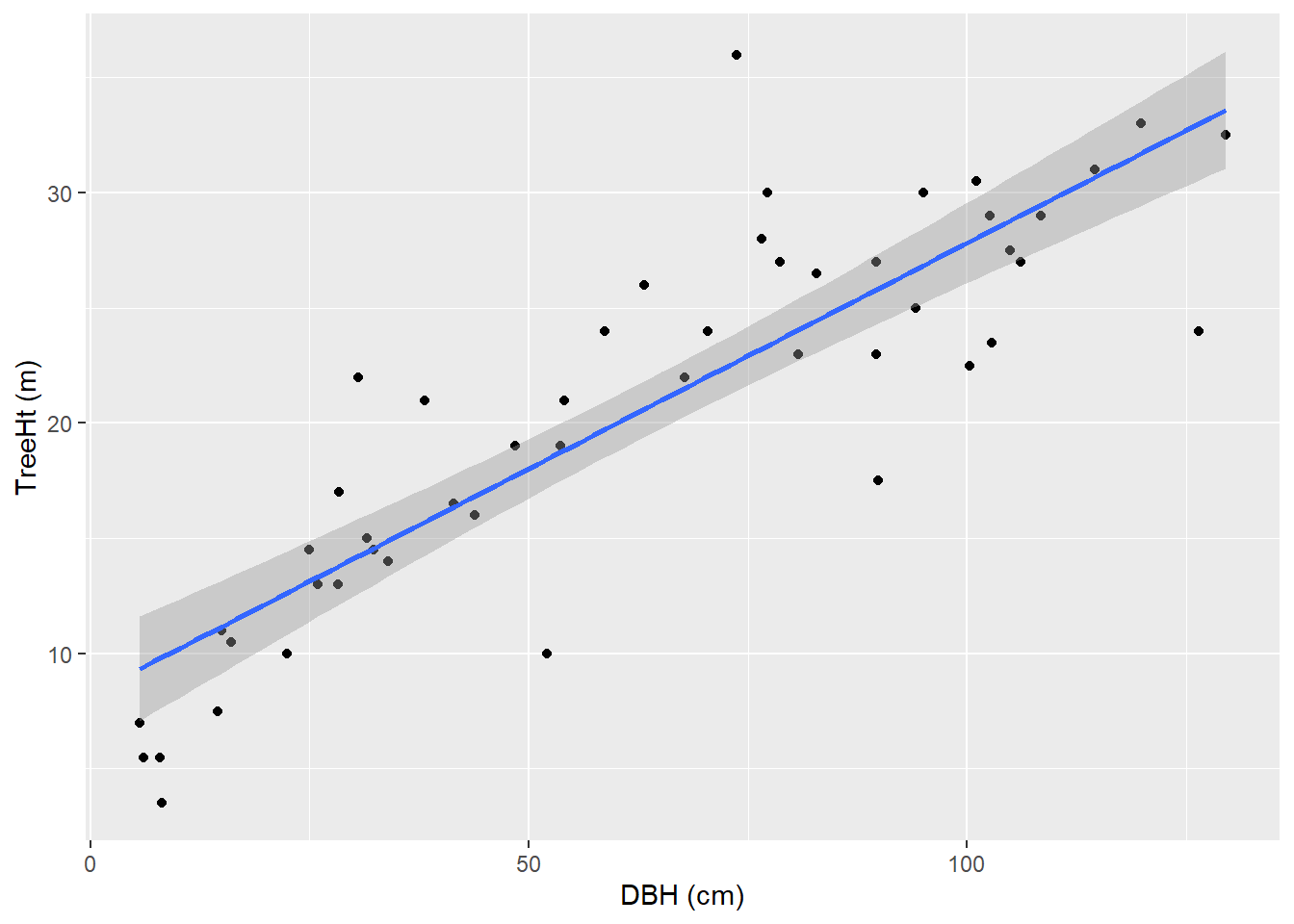
A value of 0.38 is not great. Let’s see if we can get a better match with diameter at breast height, or DBH:
Here you might notice is that we added an argument, method="lm", to the geom_smooth function. This is saying that, rather than use the default loess smoother, we want to use a linear model. This lets ggplot create a line from a linear model. From this plot, it looks like there is a pretty good relationship between these two variables.
However, we still want to assess the data using a correlation:
Warning in cor.test.default(treeDataNC$`DBH (cm)`, treeDataNC$`TreeHt (m)`, :
Cannot compute exact p-value with ties
    Spearman's rank correlation rho

data:  treeDataNC$`DBH (cm)` and treeDataNC$`TreeHt (m)`
S = 2571.2, p-value = 5.943e-16
alternative hypothesis: true rho is not equal to 0
sample estimates:
     rho
0.868814
The Spearman test says we can’t rule out a relationship (no surprise), and there is a stronger positive relationship than what we saw before (again, not surprising).
Call:
lm(formula = `TreeHt (m)` ~ `DBH (cm)`, data = treeDataNC)

Residuals:
    Min      1Q  Median      3Q     Max
-9.0051 -2.0312 -0.0645  2.0496 13.3311

Coefficients:
            Estimate Std. Error t value Pr(>|t|)
(Intercept)  8.24141    1.20525   6.838 1.44e-08 ***
`DBH (cm)`   0.19576    0.01667  11.740 1.41e-15 ***
---
Signif. codes:  0 '***' 0.001 '**' 0.01 '*' 0.05 '.' 0.1 ' ' 1

Residual standard error: 4.214 on 47 degrees of freedom
Multiple R-squared:  0.7457,    Adjusted R-squared:  0.7403
F-statistic: 137.8 on 1 and 47 DF,  p-value: 1.411e-15
This gives us an improved R-squared, suggesting that more of the variability in this dataset is explained by the model.
Going further
This really only scratches the surface when it comes to modeling with data. Linear models are very useful, but also limited because many relationships are not linear. For example, think about the relationship between how long it would take to clean your house and the number of people helping. At lower numbers of people, the amount of time is likely to decrease as you have more assistance; but after a certain point, the house becomes too crowded for anyone to move, and the presence of so many people will create more mess than you can keep up with.
One thing to keep an eye out for is instances where the response variable is not normally distributed across the predictor values. For example, if you have a binary response variable (0 or 1), it is not possible to consider this normally distributed. The Generalized Linear Model can be accessed using the glm function, and allows you to specify a distribution other than normal in your assessment of the data.
If you’re interested in looking into doing more complex modeling, there are a number of resources out there. Here are a couple to get you started:
There is an excellent section on regression in YaRrr! The Pirate’s Guide to R by Nathaniel Phillips, including a section on using the Generalized Linear Model.
If you’re interested in doing more complex modeling and integrating modeling within the tidyverse workflow, I highly recommend Tidy Modeling with R by Max Kuhn and Julia Silge. The functions take on a very different structure, but once mastered can be very powerful for modeling data.