3  Tidying data

In class, we discussed the principles of tidy data:

• each variable is stored in its own column

• each observation is stored in its own row

• each cell contains a unique value

These seem pretty straightforward, but in fact these simple rules are broken quite regularly, with data stored in column names, or multiple data types stored in a single column, or variables stored in both rows and columns. The tidyr package provides some key functions for dealing with these kinds of issues.

3.0.1 Pivot_longer

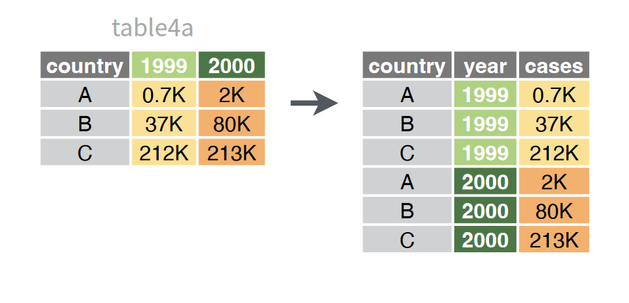
Oftentimes, categorical information you want to use is actually stored in the names of columns. To deal with this, we can gather the data in these columns into two columns: one with the column names, and another with their associated values.

In the tree dataset, for example, the last 8 columns are values for DBH recorded across multiple stems (up to 8). Not every tree will have these, so the table uses -1 to indicate an absence of stems. We can use pivot_longer to turn each of these columns into a value in a single column:

stemData<-pivot_longer(
  data=treeData,
  cols=dbh1:dbh8,
  names_to="stemNum",
  values_to="dbhMeasure"
)

Here’s a breakdown of the arguments being used here:

1. data is the table being pivoted (in this case, treeData)

2. cols is the columns where the names are going to be converted to data (in this case, columns dbh1 to dbh8 (you could substitute a vector of columns names if they aren’t in sequential order)

3. names_to provides a name for a new column where the names are going to be stored as a data

4. values_to provides a name for a new column where the values from the columns we are converting will go.

Running this code, you can see the effect. While we’re at it, we might want to eliminate the letters “dbh” from the stem number values. We can do this by adding an additional argument: names_prefix.

stemData<-pivot_longer(
  data=treeData,
  cols=dbh1:dbh8,
  names_to="stemNum",
  values_to="dbhMeasure",
  names_prefix = "dbh"
)

Now when we look at our data, we have a few less variables to deal with but a considerably larger number of observations:

stemData

# A tibble: 115,896 × 35
   DbaseID Region City   Source TreeID Zone  `Park/Street` SpCode ScientificName
     <dbl> <chr>  <chr>  <chr>   <dbl> <chr> <chr>         <chr>  <chr>         
 1       1 InlVal Modes… Motow…      1 Nurs… Nursery       ACSA1  Acer sacchari…
 2       1 InlVal Modes… Motow…      1 Nurs… Nursery       ACSA1  Acer sacchari…
 3       1 InlVal Modes… Motow…      1 Nurs… Nursery       ACSA1  Acer sacchari…
 4       1 InlVal Modes… Motow…      1 Nurs… Nursery       ACSA1  Acer sacchari…
 5       1 InlVal Modes… Motow…      1 Nurs… Nursery       ACSA1  Acer sacchari…
 6       1 InlVal Modes… Motow…      1 Nurs… Nursery       ACSA1  Acer sacchari…
 7       1 InlVal Modes… Motow…      1 Nurs… Nursery       ACSA1  Acer sacchari…
 8       1 InlVal Modes… Motow…      1 Nurs… Nursery       ACSA1  Acer sacchari…
 9       2 InlVal Modes… Motow…      2 Nurs… Nursery       BEPE   Betula pendula
10       2 InlVal Modes… Motow…      2 Nurs… Nursery       BEPE   Betula pendula
# ℹ 115,886 more rows
# ℹ 26 more variables: CommonName <chr>, TreeType <chr>, address <chr>,
#   street <chr>, side <chr>, cell <dbl>, OnStreet <chr>, FromStreet <chr>,
#   ToStreet <chr>, Age <dbl>, `DBH (cm)` <dbl>, `TreeHt (m)` <dbl>,
#   CrnBase <dbl>, `CrnHt (m)` <dbl>, `CdiaPar (m)` <dbl>,
#   `CDiaPerp (m)` <dbl>, `AvgCdia (m)` <dbl>, `Leaf (m2)` <dbl>,
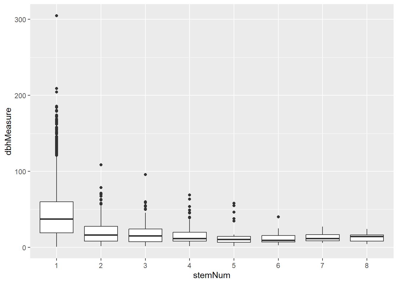
#   Setback <dbl>, TreeOr <dbl>, CarShade <dbl>, LandUse <dbl>, Shape <dbl>, …

What this data allows us to do more easily is use stem number itself as a variable. For example, we can now plot a boxplot to show how these vary in terms of DBH measurements:

stemData2<-filter(stemData,dbhMeasure>-1)
ggplot(stemData2,aes(x=stemNum,y=dbhMeasure)) +
  geom_boxplot()

3.0.2 Pivot_wider

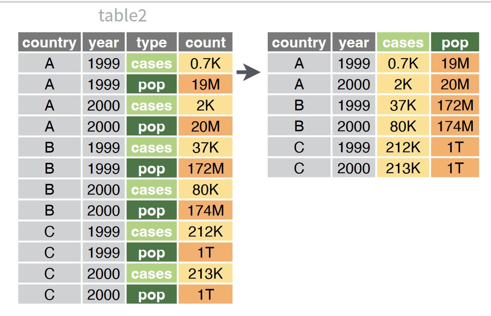
Pivoting wider involves taking data that is stored in a single column and spreading it across multiple columns.

Here, we’ll use it to convert out tree data back into the format we’re used to:

treeWide<-pivot_wider(
  data=stemData,
  names_from=stemNum,
  values_from=dbhMeasure
)
treeWide

# A tibble: 14,487 × 41
   DbaseID Region City   Source TreeID Zone  `Park/Street` SpCode ScientificName
     <dbl> <chr>  <chr>  <chr>   <dbl> <chr> <chr>         <chr>  <chr>         
 1       1 InlVal Modes… Motow…      1 Nurs… Nursery       ACSA1  Acer sacchari…
 2       2 InlVal Modes… Motow…      2 Nurs… Nursery       BEPE   Betula pendula
 3       3 InlVal Modes… Motow…      3 Nurs… Nursery       CESI4  Celtis sinens…
 4       4 InlVal Modes… Motow…      4 Nurs… Nursery       CICA   Cinnamomum ca…
 5       5 InlVal Modes… Motow…      5 Nurs… Nursery       FRAN_R Fraxinus angu…
 6       6 InlVal Modes… Motow…      6 Nurs… Nursery       FREX_H Fraxinus exce…
 7       7 InlVal Modes… Motow…      7 Nurs… Nursery       FRHO   Fraxinus holo…
 8       8 InlVal Modes… Motow…      8 Nurs… Nursery       FRPE_M Fraxinus penn…
 9       9 InlVal Modes… Motow…      9 Nurs… Nursery       FRVE_G Fraxinus velu…
10      10 InlVal Modes… Motow…     10 Nurs… Nursery       GIBI   Ginkgo biloba 
# ℹ 14,477 more rows
# ℹ 32 more variables: CommonName <chr>, TreeType <chr>, address <chr>,
#   street <chr>, side <chr>, cell <dbl>, OnStreet <chr>, FromStreet <chr>,
#   ToStreet <chr>, Age <dbl>, `DBH (cm)` <dbl>, `TreeHt (m)` <dbl>,
#   CrnBase <dbl>, `CrnHt (m)` <dbl>, `CdiaPar (m)` <dbl>,
#   `CDiaPerp (m)` <dbl>, `AvgCdia (m)` <dbl>, `Leaf (m2)` <dbl>,
#   Setback <dbl>, TreeOr <dbl>, CarShade <dbl>, LandUse <dbl>, Shape <dbl>, …

3.0.3 Separate

The seperate function takes columns where there is more than one piece of information and breaks it up into multiple columns. For example, let’s say we wanted separate columns for the genus and species of the trees:

treeDataSep<-separate(
  data=treeData,
  col=ScientificName,
  into=c("Genus","Species"),
  sep=" ",
  extra="drop")
treeDataSep

# A tibble: 14,487 × 42
   DbaseID Region City    Source TreeID Zone  `Park/Street` SpCode Genus Species
     <dbl> <chr>  <chr>   <chr>   <dbl> <chr> <chr>         <chr>  <chr> <chr>  
 1       1 InlVal Modest… Motow…      1 Nurs… Nursery       ACSA1  Acer  saccha…
 2       2 InlVal Modest… Motow…      2 Nurs… Nursery       BEPE   Betu… pendula
 3       3 InlVal Modest… Motow…      3 Nurs… Nursery       CESI4  Celt… sinens…
 4       4 InlVal Modest… Motow…      4 Nurs… Nursery       CICA   Cinn… campho…
 5       5 InlVal Modest… Motow…      5 Nurs… Nursery       FRAN_R Frax… angust…
 6       6 InlVal Modest… Motow…      6 Nurs… Nursery       FREX_H Frax… excels…
 7       7 InlVal Modest… Motow…      7 Nurs… Nursery       FRHO   Frax… holotr…
 8       8 InlVal Modest… Motow…      8 Nurs… Nursery       FRPE_M Frax… pennsy…
 9       9 InlVal Modest… Motow…      9 Nurs… Nursery       FRVE_G Frax… veluti…
10      10 InlVal Modest… Motow…     10 Nurs… Nursery       GIBI   Gink… biloba 
# ℹ 14,477 more rows
# ℹ 32 more variables: CommonName <chr>, TreeType <chr>, address <chr>,
#   street <chr>, side <chr>, cell <dbl>, OnStreet <chr>, FromStreet <chr>,
#   ToStreet <chr>, Age <dbl>, `DBH (cm)` <dbl>, `TreeHt (m)` <dbl>,
#   CrnBase <dbl>, `CrnHt (m)` <dbl>, `CdiaPar (m)` <dbl>,
#   `CDiaPerp (m)` <dbl>, `AvgCdia (m)` <dbl>, `Leaf (m2)` <dbl>,
#   Setback <dbl>, TreeOr <dbl>, CarShade <dbl>, LandUse <dbl>, Shape <dbl>, …

The arguments here should look familiar, but a couple may be worth discussing. The sep argument gives the symbol that separates the two sections. Here, the genus and species are separated by a single space, so we include that in quotes. The extra argument gives instructions on what to do with any extra data. If you look at the original tree data, you can see some scientific names have more than two parts. In this case, let’s assume we’re not too fussy about that, so we use the argument “drop” to get rid of it.

3.0.4 Unite

Unite is the opposite of separate. It simply takes two columns and puts them together, like so:

treeDataUnite<-unite(
  data=treeDataSep,
  col="SciName",
  Genus:Species,
  sep=" ",
  remove=TRUE)
treeDataUnite

# A tibble: 14,487 × 41
   DbaseID Region City        Source   TreeID Zone  `Park/Street` SpCode SciName
     <dbl> <chr>  <chr>       <chr>     <dbl> <chr> <chr>         <chr>  <chr>  
 1       1 InlVal Modesto, CA Motown2…      1 Nurs… Nursery       ACSA1  Acer s…
 2       2 InlVal Modesto, CA Motown2…      2 Nurs… Nursery       BEPE   Betula…
 3       3 InlVal Modesto, CA Motown2…      3 Nurs… Nursery       CESI4  Celtis…
 4       4 InlVal Modesto, CA Motown2…      4 Nurs… Nursery       CICA   Cinnam…
 5       5 InlVal Modesto, CA Motown2…      5 Nurs… Nursery       FRAN_R Fraxin…
 6       6 InlVal Modesto, CA Motown2…      6 Nurs… Nursery       FREX_H Fraxin…
 7       7 InlVal Modesto, CA Motown2…      7 Nurs… Nursery       FRHO   Fraxin…
 8       8 InlVal Modesto, CA Motown2…      8 Nurs… Nursery       FRPE_M Fraxin…
 9       9 InlVal Modesto, CA Motown2…      9 Nurs… Nursery       FRVE_G Fraxin…
10      10 InlVal Modesto, CA Motown2…     10 Nurs… Nursery       GIBI   Ginkgo…
# ℹ 14,477 more rows
# ℹ 32 more variables: CommonName <chr>, TreeType <chr>, address <chr>,
#   street <chr>, side <chr>, cell <dbl>, OnStreet <chr>, FromStreet <chr>,
#   ToStreet <chr>, Age <dbl>, `DBH (cm)` <dbl>, `TreeHt (m)` <dbl>,
#   CrnBase <dbl>, `CrnHt (m)` <dbl>, `CdiaPar (m)` <dbl>,
#   `CDiaPerp (m)` <dbl>, `AvgCdia (m)` <dbl>, `Leaf (m2)` <dbl>,
#   Setback <dbl>, TreeOr <dbl>, CarShade <dbl>, LandUse <dbl>, Shape <dbl>, …

The last argument in this case, remove, takes away the now redundant columns of Genus and Species.

Try it yourself!

Use the separate and unite functions to do the following:

• In the tree dataset, create separate columns for city and state

• In the Sacramento dataset, combine the latitude and longitude columns