3  Customizing Labels

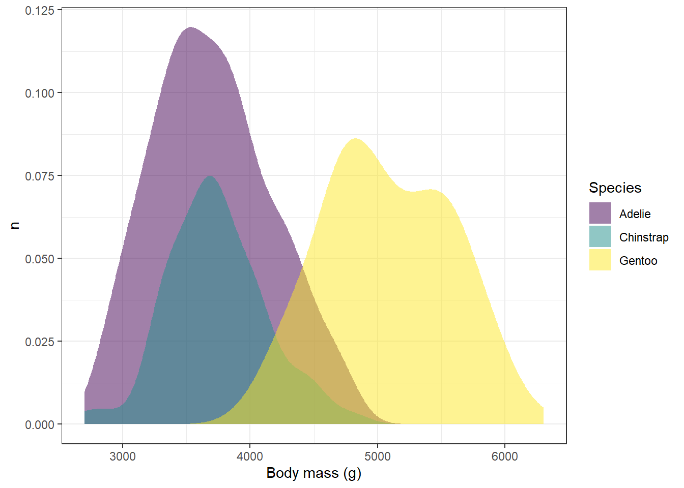
3.0.1 Putting labels on things: the annotate function

Returning to our penguin plot:

ggplot(drop_na(penguins,body_mass_g,species),aes(x=body_mass_g,y=after_stat(count),fill=species))+
  geom_density(alpha=0.5,color=NA) +
  scale_fill_viridis_d(option="viridis") +
  theme_bw() +
  labs(x="Body mass (g)",y="n",fill="Species")

Let’s say that we’re finding the legend on the right hand side to be kind of distracting. We could use the show.legend

ggplot(drop_na(penguins,body_mass_g,species),aes(x=body_mass_g,y=after_stat(count),fill=species))+
  geom_density(alpha=0.5,color=NA,show.legend = FALSE) +
  scale_fill_viridis_d(option="viridis") +
  theme_bw() +
  labs(x="Body mass (g)",y="n",fill="Species")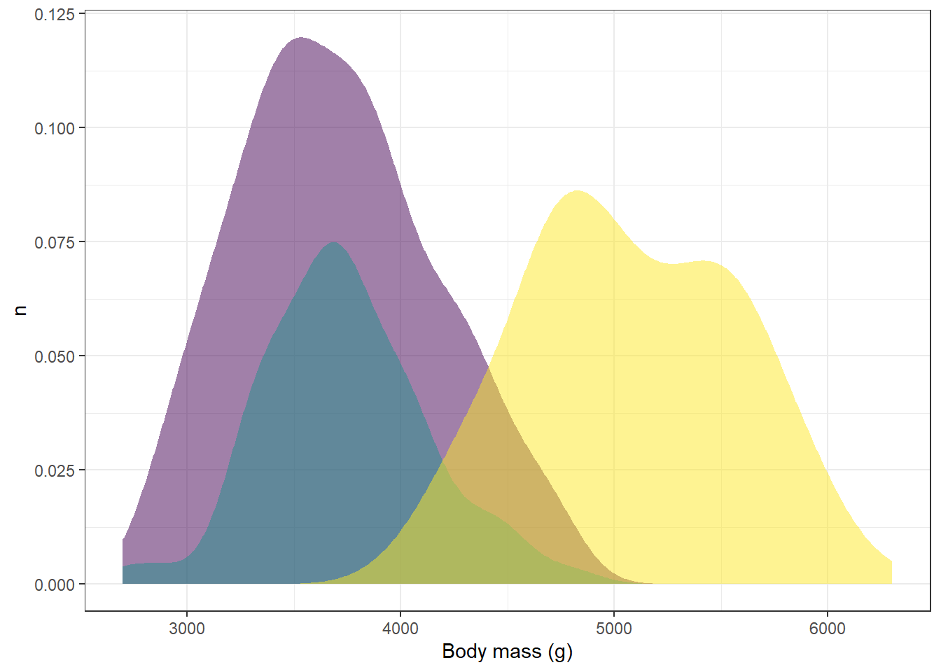 

However, now we don’t know what distribution corresponds to what species. One way we could deal with this would be to add labels that correspond with the distributions in the image. We can add individual labels to items using the annotate function:

ggplot(drop_na(penguins,body_mass_g,species),aes(x=body_mass_g,y=after_stat(count),fill=species))+
  geom_density(alpha=0.5,color=NA,show.legend = FALSE) +
  scale_fill_viridis_d(option="viridis") +
  theme_bw() +
  labs(x="Body mass (g)",y="n",fill="Species") +
  annotate(geom="label",x=3500,y=0.1,label="Adelie") +
  annotate(geom="label",x=3600,y=0.05,label="Chinstrap") +
  annotate(geom="label",x=5000,y=0.04,label="Gentoo")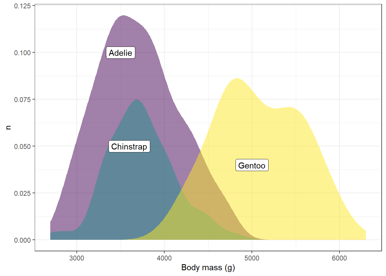

Let’s break down the arguments here for each of these annotate functions:

• geom This tells us what kind of geometry to use. In this case, we’ll use the label geom, but other options are arrows, line segments, points, etc.

• x, y This gives the x and y position for the center of the label

• label This is the text that will be included in the label

These look pretty good. But let’s say we want to plot the labels using the same colors from the viridis palette. Annotation colors can be modified using the color function, but first we need to know what our colors names are. We did this earlier with the show_col and viridis_pal functions, but since we’re only looking at three categories here, we only need to request three colors:

show_col(viridis_pal()(3))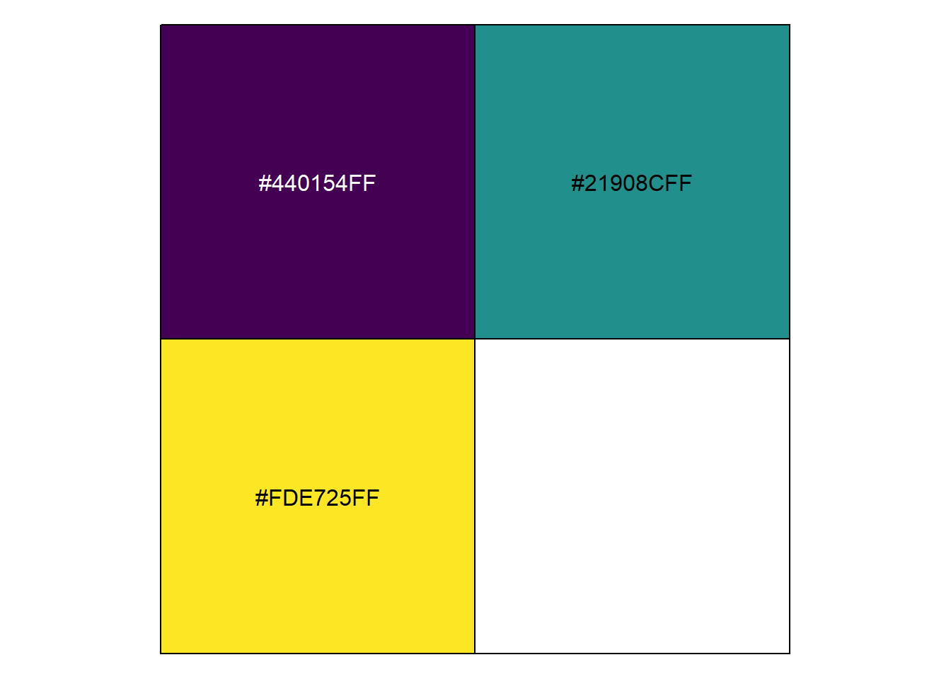

These are our hexidecimal codes for the colors we’re using. We can add them to the annotate function using the color argument and giving each one as a character value (e.g., “#440154FF”), but typing each of these codes out would be pain.

Another way we could do this would be to store them as a vector of values by skipping the show_col function:

myCols<-viridis_pal()(3)
myCols

[1] "#440154FF" "#21908CFF" "#FDE725FF"

Remember way back when we learned about vectors and how to access individual values? That’s right, we’re going to use square brackets ([])! We can use the indices of each value in the myCols vector for each of the annotate calls:

ggplot(drop_na(penguins,body_mass_g,species),aes(x=body_mass_g,y=after_stat(count),fill=species))+
  geom_density(alpha=0.5,color=NA,show.legend = FALSE) +
  scale_fill_viridis_d(option="viridis") +
  theme_bw() +
  labs(x="Body mass (g)",y="n",fill="Species") +
  annotate(geom="label",x=3500,y=0.1,label="Adelie",color=myCols[1]) +
  annotate(geom="label",x=3600,y=0.05,label="Chinstrap",color=myCols[2]) +
  annotate(geom="label",x=5000,y=0.04,label="Gentoo",color=myCols[3])

3.0.2 Dealing with math in the labels: the bquote function

What if you want to put non-standard characters into labels, like subscripts, superscripts, or Greek letters? For this example, we’ll draw on the scat dataset from the modeldata package:

library(modeldata)

Attaching package: 'modeldata'

The following object is masked from 'package:palmerpenguins':

    penguins

ggplot(drop_na(scat,d13C,d15N),aes(x=d13C,y=d15N)) +
  geom_point()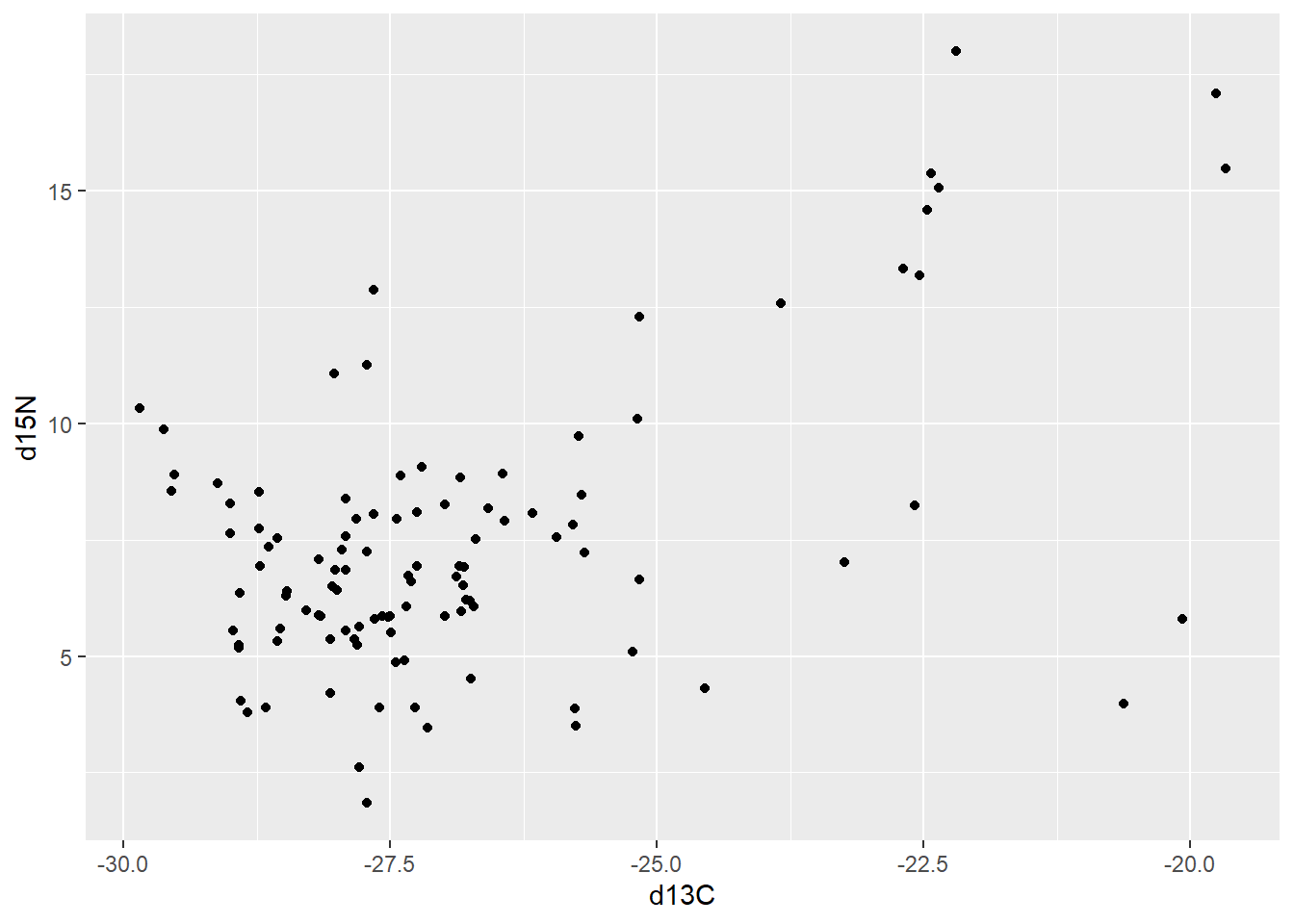 

Here, what we are showing is the relationship between two stable isotope concentrations: carbon-13 and nitrogen-15. These isotopes are used to evaluate and compare animal diets, and their values are typically expressed using superscripted numbers before the periodic symbol for the element (here C for carbon and N for nitrogen), and the Greek symbol delta indicating that it is differenced from a reference standard. For example:

\[ \delta^{13}C \]

and

\[ \delta^{15}N \] If we want to modify the labels on the axes, we can change it using the bquote function:

library(modeldata)

ggplot(drop_na(scat,d13C,d15N),aes(x=d13C,y=d15N)) +
  geom_point() +
  labs(x=bquote(delta^13~C),y=bquote(delta^15~N))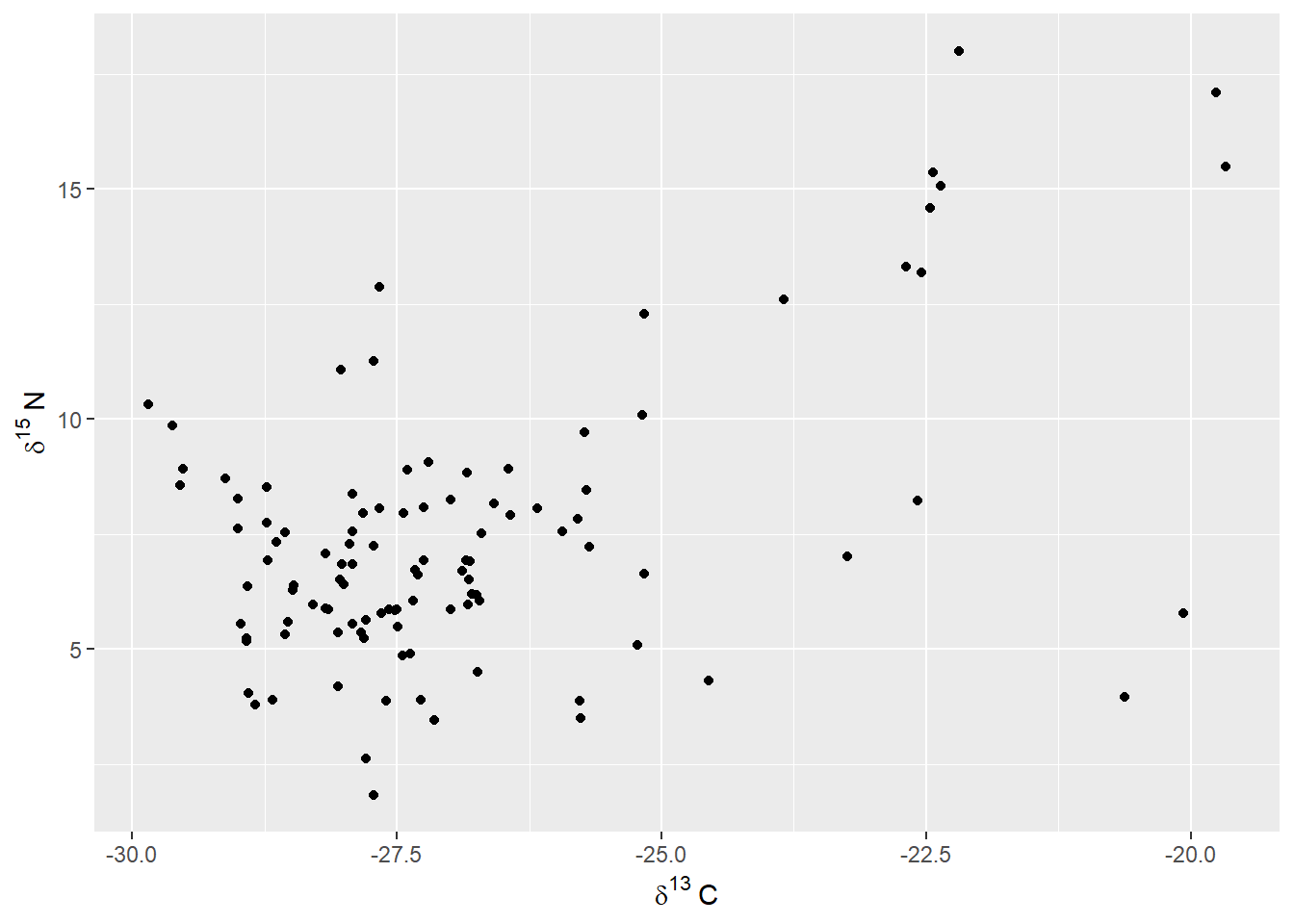

Here, rather than give a single text value, we provide bquote with an expression. For example, where it reads delta^13~C, this is saying combine the Greek letter delta with a superscripted 13 (^13) and then add a capital letter C at the end. The tilde (~) here is used when you need to transition between different parts of the phrase that don’t fit together naturally in sequence; for example, the superscripted 13 and the letter C.

Try it yourself!

Using the Sacramento data, make a boxplot of square footage by property type, then try using bquote to create a label that shows the sqft variable as ft\(^2\).