1 Introducing code notebooks and Quarto
Code notebooks are software tools that combine code, text, and outputs in a single document. They are based on the notion of Literate Programming, first promoted by Donald Knuth, where code is written in a way where it can also be understood in a human language. This approach was originally developed to address a few different problems:
Spelling out what code does as it is written it will force the author to consider whether it might be done in a more effective way.
Combining code with human-readable text allows researchers using other programing languages to understand the logic and more easily translate between languages
As code ages, having a plain-text explanation of the code’s operation helps protect against its complete loss to obselesence
In addition, contemporary code notebooks have been found to have several additional benefits:
Code notebooks encourage collaboration between you and other researchers, enabling ideas to be re-used and built upon
Code notebooks can be translated into different kinds of documents, which can be tailored to reach different audiences (e.g., researchers, policymakers, community stakeholders, etc.)
Code notebooks provide clear documentation of the data science process, allowing researchers to quickly recall the thinking behind different coding decisions
Since we’re discussing advantages of notebooks, it’s probably also a good time to mention situations when they would not be useful. Code that is made to operate For example, if you’re writing a set of computationally-intensive climate simulations that have multiple iterative loops and/or need to be distributed across multiple machines, having the code having a code structure that runs in parts and/or stops regularly between text sections doesn’t make a lot of sense.
That said, much of the business of data science often involves work that occurs in discrete parts, including:
cleaning and tidying datasets
transforming data structures
visualizing patterns in data
modeling relationships between data
communicating about findings
Code notebooks are well-situated to integrate with these activities. In this section, we’ll go over the basics of creating a code notebook in Quarto.
1.0.1 Creating a Quarto document
Quarto documents can be created directly in RStudio, and will open in the Source tab like an R script. Go to the File dropdown menu, select New File, and then Quarto Document. You should see a dialogue box open that looks something like this:
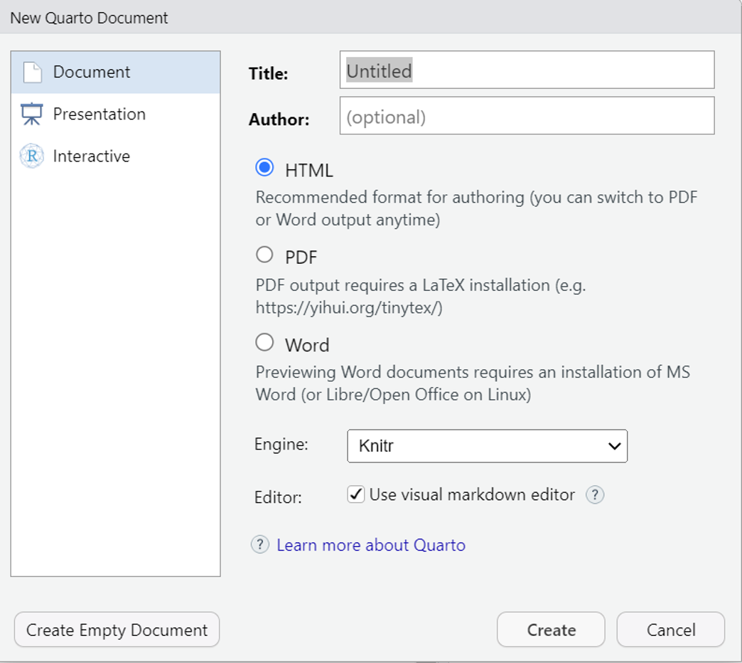
Here you can set the document name and author, the kind of project you want to create, the kind of file you want to publish the output, and a few other options.
For this lab, we’re going to start off with a Quarto Document. Name it anything you like, though it would help to name it something that associates it with the lab. List yourself as the author. And for now, we’ll use the default settings for output (HTML1), engine (Knitr), and we’ll use the visual editor. Click Create. You should now see a new document that looks something like this:
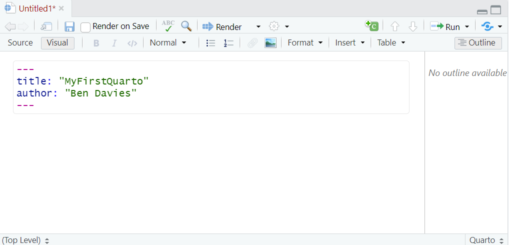
Be aware that creating the document will not save your new document as a file. Notice when the tab is created, the document is called Untitled1. Take this opportunity to save the file by going to the File dropdown menu, select Save As, and save your document to your working directory. This should now appear in your Files tab as a Quarto Markdown (.qmd) file.
Looking at the document, it probably looks like a blank script file except for a few lines at the top bracketed by three hyphens (---). These lines are called a YAML block. They define some global parameters for the document, which so far include the title and author. There are a lot more parameters you might set here; we’ll discuss this shortly.
1.0.2 Editing a Quarto document
Quarto documents might include a number of different elements, but three of the most typical are headers, text, and code chunks. We’ll look at how to add each of these to our presently empty Quarto document.
1.0.2.1 Headers
Headers (or headings) are text that breaks up sections and subsections of the document. Headers are given in different levels, which define the size of the text used in the header. In this document, you can see a few different levels of headers:
Header 2
1.1 Introducing code notebooks and Quarto
Header 3
1.1.1 Editing a Quarto document
Header 4
1.1.1.1 Headers
You can change the heading by using a dropdown menu in the editor bar at the top of the document:

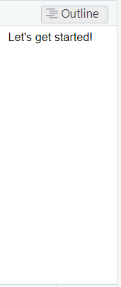
Add a header to your Quarto document that reads “Let’s get started”, and set it to the Header 3 level.
Headers also allow for an in-built outlining, which you can see at right. This can be used to jump between sections as your document grows:
1.1.1.2 Text
Text is simply that: text you add to your document. You can make modifications to the text style using buttons on the, much like a word processor like MS Word.

The first two should be familiar:
Bold
Italics
The last option, </>, indicates that you want the text to be rendered in the font used for code:
Code
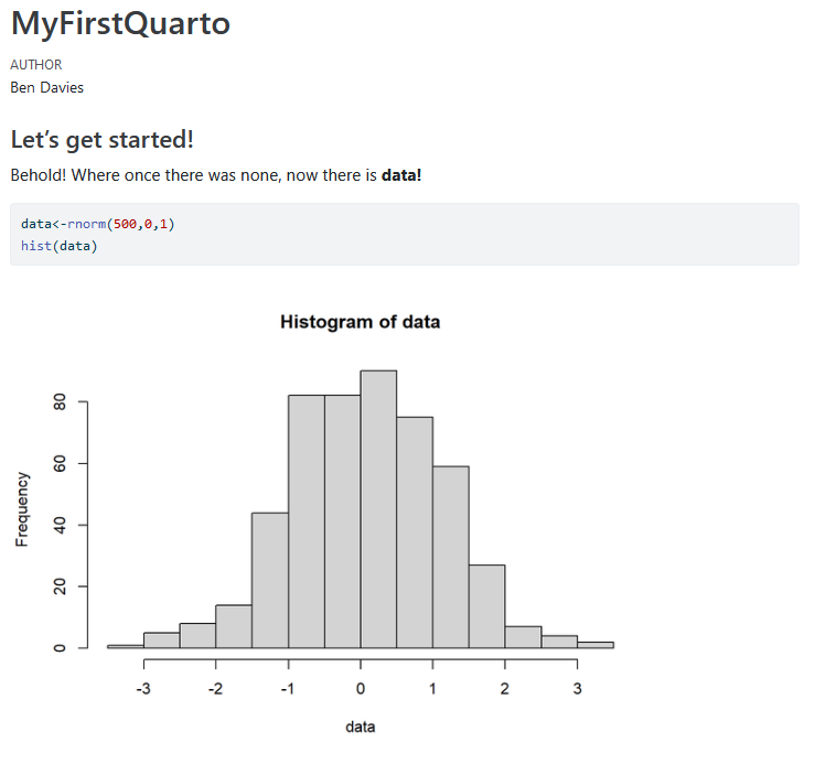
Add some text that totally oversells the simple R operation you’re going to do next. Modify some element of it with bolding, italics, or code formatting.
1.1.1.3 Code Chunks
Code chunks are pretty much what they sound like: a section of code run separately from the rest of the code. You can add a code chunk using this button on the editor bar:

A blank chunk will look something like this:
![]()
Anything added to this grey block after the {r} will work as if it were part of an R script. Y
Add a code chunk to your document, and include some code in this that uses rnorm to generate a vector of 500 values with a mean of 0 and a standard deviation of 1, then plots these as a histogram. You can see the result by pressing the green triangle (play) button at the top right of the chunk.
1.1.2 Rendering a Quarto document
When we’re ready to share our work, we need to render the entire thing into a document. To do this, we use the Render button:

What this does is first takes the entire document and, via the knitr package, puts together all of our different elements as a general markdown file which includes the executed code and any graphics it generates. The markdown file is then translated into the file format we’re trying to create using pandoc software.
Remember at the outset that we used the default HTML as our output. An HTML document is the kind of document used to create webpages, so this process will take our and create a webpage.
Click Render, and you should see the Console pane switch to the Background Jobs tab. This should iterate through some text indicating which part of the If all goes well, your default browser should open up displaying your document:
If you look at the search bar, it references localhost rather than a URL (e.g., http://www.tufts.edu). This is because the HTML document you’re viewing is currently currently on your hard drive rather than on a file server. However, if you look in your Files tab, you should see that you now have two new things: an HTML (.html) file and a corresponding folder with the suffix “_files”. If you were to copy these to a file server, they would be visible as a website that others can access.
Some common issues that may arise when rendering your Quarto document:
If you reference a function from package that is not loaded in your document, it will create an error and stop the process. In this case, just add a code chunk with the
libraryfunction (e.g.,library(tidyverse)). Don’t include calls toinstall.packagesin the document! The rendered document will include the packages you’re using as files to be included.If you try and run some code that produces an error, it will notify you and stop the process. Go back to that section and fix the error.
If you’re storing things on a cloud-based drive, this can sometimes interfere when it syncs.
Add a second header to your Quarto document entitled “Let’s get continuing!”, include some text that touts your data science prowess, and use it to produce a histogram from the same data using different arguments for breaks and col. Keep in mind that if you already stored your vector of random values as an object, you won’t need to run rnorm again.
To publish directly to PDF, we need to make sure that you have a distribution of the typesetting software LaTeX installed (incidentally, Knuth is the author of LaTeX’s progenitor, TeX). You can do this by running
install.packages("tinytex")from the command line.↩︎