library(tidyverse)
abalone<-read_csv("data/abalone.csv")
abalone2 Looking under the hood
Most of the operations we just used to create our document took place in the editor bar:

This bar is included as part of Quarto’s visual editor. The visual editor lets you modify a document using a WYGIWYM (What You See Is What You Mean) interface, so the things that you see in the document (e.g., bolding, headings, code outputs) are rendered more or less as you would expect them to appear, but with some markings and controls embedded in the document (for example, the play button on the code chunk).
The Quarto document itself is actually a script written using Markdown language, which is used for formatting documents that are a mix of text and executable code. The Visual Editor takes these elements and shows them to you in a way that lets you assess their visual look, but the actual .qmd file you’re creating looks a little different…
2.0.1 Quarto source editor
At the left side of the editor bar, you can toggle between the visual editor and the source editor:

What you see should now should look similarly to the document we were working on, except that the formatting has been removed. The source shows what the .qmd file looks like in reality: a text file with some additional In fact, if we took this out of RStudio and opened it in a text editor like Notepad, it would look something like this:
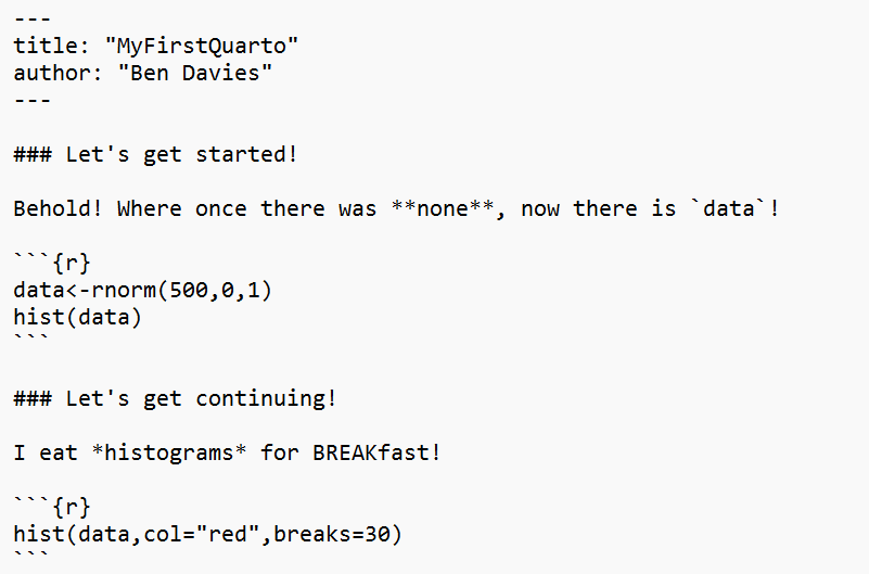
What you’re seeing here is an example of Markdown, which is a text file where particular sequences of symbols are translated into text formatting and code chunks. For example:
Hash marks (
###) are used to indicate header levelBold text is surrounded by two asterisks
**Text in italics will be surrounded by single asterisks
*Text in
codeformat will be surrounded by single backticks`Code chunks begin and end with three backticks
```Code chunks will usally begin with curly braces containing the language being used (
{r})
Markdown enables the literal programming approach because, as you can see, even with thie additional symbols this document is still very much readable.
Pay particular attention to what’s happening inside the code chunk. What this section is doing is telling Markdown (and subsequently Pandoc) that this is meant to be read as executable code. As the final output is being rendered, this code will be processed and any outputs will be added to the document.
Try it yourself!
Add to the document you’ve created using the Source editor.
Add a third header called “This is the third section!”
Add some text to further emphasize your data science skills, and modify it with bolding, italics, or code formatting (make sure not to attempt this inside a code chunk!)
Add a code chunk that include code that uses
runifto generate two vectors of 500 random values between 0 and 1, and then plots them using theplotfunction.
You can edit your document in the source code editor, then switch back to the visual editor to see what your document will look like. Some more complex elements (for example, adding raw HTML code) will not show up formatted correctly in the visual editor, but will when the document is rendered.
You might be asking yourself why you would ever use the Source when you can use the Visual Editor. The short answer is that, like other word processing software, there’s room for software error, especially when a document becomes large or formatting becomes very complex (alternating between code formatting and italics in a single line, for example). If something doesn’t look right, you can use the source editor to check what’s going on underneath the hood.
2.0.2 Modifying the YAML header
The YAML header is where you can include settings that you want applied across the whole document. For example, here I’ve added a few
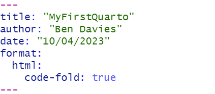
Here, I’ve added a field for the date, and changed the way the HTML document using code-fold, which will take the code chunks and make them hideable/expandable. Feel free to modify your YAML to include the same options.
There are a lot of ways you can modify the YAML header to change the way the document behaves, including adding tables of contents and bibliographies from bibliography managers like EndNote and Zotero. We won’t go into these in too much depth for the moment; if you’re interested in how these work, you can read more about them here. There are also ways to apply settings to individual sections and code chunks. We’ll look at a few of these in the next section.
2.0.3 File handling with Quarto Documents
Often, the work that we are documenting in a Quarto document will involve some external dataset: for example, data stored in a .csv file. We’ve dealt with importing data from outside of R before.
The same is true when working in a Quarto document. The default working directory for a Quarto document is the directory where it is saved, and file paths are considered relative to that position.
Download the abalone dataset from canvas and save it in a subdirectory within your working directory called “data”. Then you can create a new code chunk with the following:
When you do this yourself, you should see two different windows here: one with the messages that come up when you call the tidyverse library and use the read_csv function, and another displaying a table with the abalone data. Our Quarto document now has access to the abalone data.
An important caveat here: if you want to share a Quarto document that is using an external data file, you need to also include that data file, ideally in the same relative location to your Quarto file. So, for example, if your data file is stored in a subdirectory called “data”, then you’d want to send both the Quarto document and that folder with the data file inside it. We’ll cover this in class later this week.